Diagnose and assess calibration

vennabers draws two kinds of graphics with base R. They answer different questions and need different data:

Kind	Shows	Needs	Functions
Fit diagnosis	the stored state of a fitted calibrator	the fit only	`plot()`
Assessment graphic	how predictions agree with outcomes	held-out pairs of truth and prediction	`corp_plot()`, `corp_decomposition_plot()`, `calibration_plot()`, `regression_plot()`

A fit diagnosis never sees new truth values, so it cannot tell whether predictions are calibrated. An assessment graphic describes the pairs it is given; draw it on assessment data kept outside training, selection and calibration. Every function returns its plotted values invisibly as a data frame, so you can check them or redraw them with another graphics system.

The examples below use a logistic model with separate training, calibration and assessment sets, as in vignette("manual-calibration", package = "vennabers").

library(vennabers)
set.seed(17)
data <- data.frame(x = rnorm(900))
data$truth <- runif(nrow(data)) < plogis(0.3 + 1.5 * data$x)
training <- data[1:300, ]
calibration <- data[301:600, ]
assessment <- data[601:900, ]

model <- glm(truth ~ x, data = training, family = binomial())
calibration_p <- predict(model, calibration, type = "response")
assessment_p <- predict(model, assessment, type = "response")
calibrator <- venn_abers(calibration$truth, calibration_p)
probability <- predict(calibrator, assessment_p)$probability

Fit diagnoses: the stored state

plot() on a fitted calibrator draws its calibration map: the lower and upper Venn-Abers values as steps and the regularized probability as a dashed line, over the uncalibrated probability on [0, 1]. which = "width" draws the Venn-Abers width upper - lower over the same scores, and which = c("map", "width") draws both.

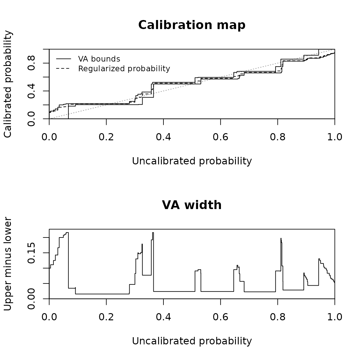
map <- plot(calibrator, which = c("map", "width"))

Calibration map and Venn-Abers width of an Inductive calibrator.

head(map)
#>         score lower     upper probability     width
#> 1 0.000000000     0 0.1000000  0.09090909 0.1000000
#> 2 0.004784115     0 0.1000000  0.09090909 0.1000000
#> 3 0.014876406     0 0.1111111  0.10000000 0.1111111
#> 4 0.021588489     0 0.1250000  0.11111111 0.1250000
#> 5 0.030187704     0 0.1428571  0.12500000 0.1428571
#> 6 0.035082226     0 0.1666667  0.14285714 0.1666667

The table has one row per stored knot plus the ends 0 and 1. Its values equal predict() at score, with loss = "log" by default; loss = "brier" draws the Brier-regularized probability instead. The width is neither a confidence level nor a nominal coverage.

A Cross calibrator overlays the map of every fold calibrator in one panel, and its table holds one block per fold:

fold <- rep(c("A", "B", "C"), length.out = nrow(calibration))
cross <- cross_venn_abers(calibration$truth, calibration_p, fold)
fold_maps <- plot(cross)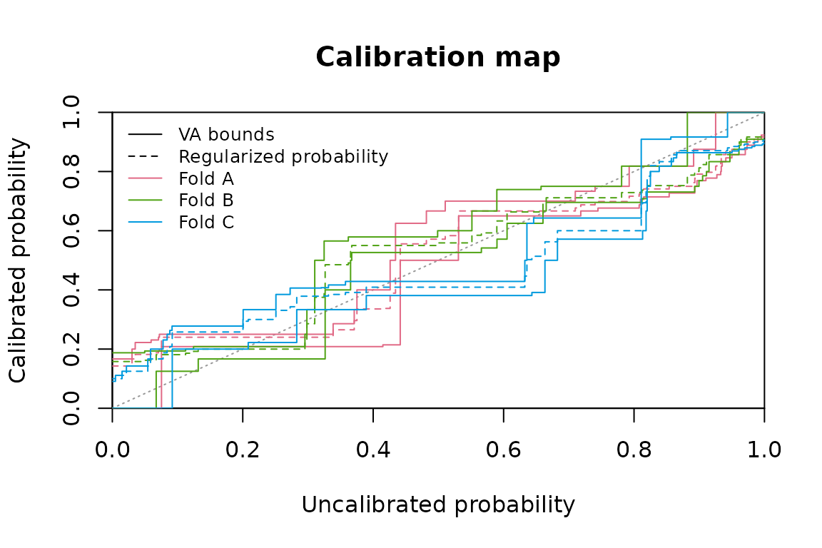

Fold maps of a Cross calibrator.

table(fold_maps$fold)
#> 
#>   A   B   C 
#> 102 102 102

The fold maps show how the fold calibrators differ at common scores. They do not describe the spread of an individual Cross prediction, which aggregates the folds.

Multiclass calibrators draw one panel per one-vs-rest class or one-vs-one pair, each the map of its own binary subproblem; the final coupling into class probabilities is not drawn. Regression calibrators draw the map over the uncalibrated prediction, with gray dashed lines at the moderated truth values a and b that bound every Venn-Abers value:

set.seed(52)
x <- runif(600, 0, 10)
regression_data <- data.frame(x = x, truth = x + sin(x) + rnorm(600, sd = 0.5))
regression_model <- lm(truth ~ x, data = regression_data[1:200, ])
uncalibrated <- predict(regression_model, regression_data)
regression <- venn_abers_regression(regression_data$truth[201:400],
                                    uncalibrated[201:400])
regression_map <- plot(regression)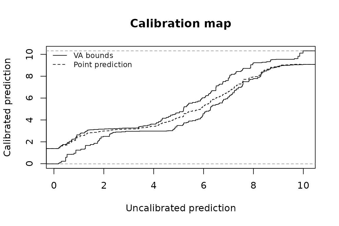

Calibration map of a regression calibrator.

For workflows, plot() also accepts a frozen fit from calibrate_workflow() and the engine fit of a trained calibrated_workflow(), extracted with workflows::extract_fit_engine(). It draws the stored Venn-Abers calibrator with the loss stored at fitting as the default. See ?plot.venn_abers for every family and for fits saved by earlier versions.

Assessment graphics: held-out pairs

CORP reliability diagrams

corp_plot() draws the CORP reliability diagram of Dimitriadis, Gneiting and Jordan (2021). Its step is the isotonic (PAV) estimate of the conditional event probability at each distinct predicted probability, compared with the dashed diagonal of perfect calibration. Unlike binned diagrams, it needs no choice of bins.

corp <- corp_plot(assessment$truth, probability, seed = 1)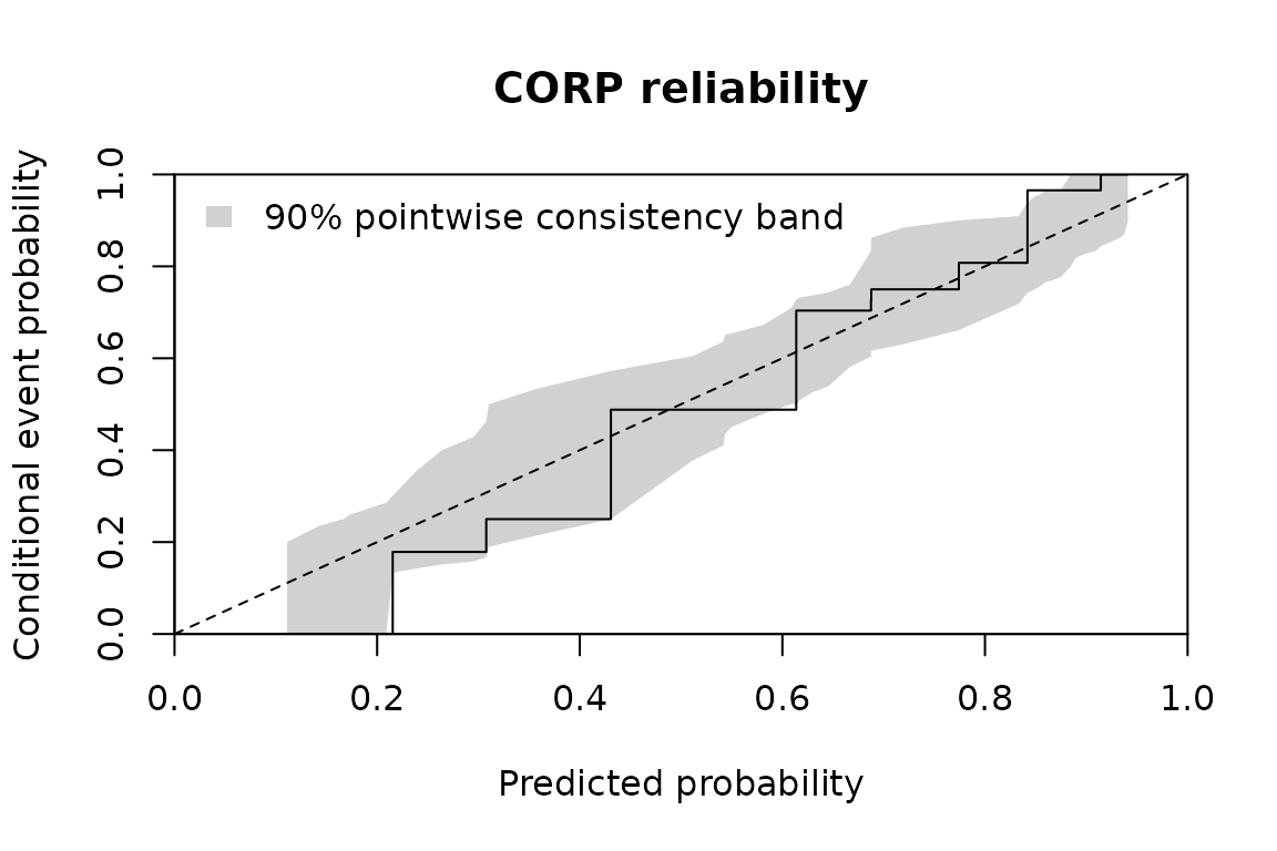

CORP reliability diagram with the consistency band.

head(corp)
#>   probability  estimate count band_lower band_upper valid_replicates
#> 1   0.1111111 0.0000000     1  0.0000000  0.2000000              643
#> 2   0.1428571 0.0000000     1  0.0000000  0.2352941              860
#> 3   0.1666667 0.0000000     2  0.0000000  0.2500000              981
#> 4   0.1720430 0.0000000     1  0.0000000  0.2587120              992
#> 5   0.2090261 0.0000000     5  0.0000000  0.2857143             1000
#> 6   0.2153846 0.1785714    49  0.1333333  0.3014329             1000
#>          band level replicates seed
#> 1 consistency   0.9       1000    1
#> 2 consistency   0.9       1000    1
#> 3 consistency   0.9       1000    1
#> 4 consistency   0.9       1000    1
#> 5 consistency   0.9       1000    1
#> 6 consistency   0.9       1000    1

The gray band is the default consistency band at level 0.9: where the CORP estimate of perfectly calibrated probabilities would fall, obtained by resampling. An estimate outside it points to miscalibration there. A seed makes the band reproducible and leaves your random stream unchanged. band = "confidence" draws an approximate pointwise band around the estimate instead, which claims no nominal coverage; see ?corp_plot for simulated coverage.

confidence <- corp_plot(assessment$truth, probability,
                        band = "confidence", seed = 1)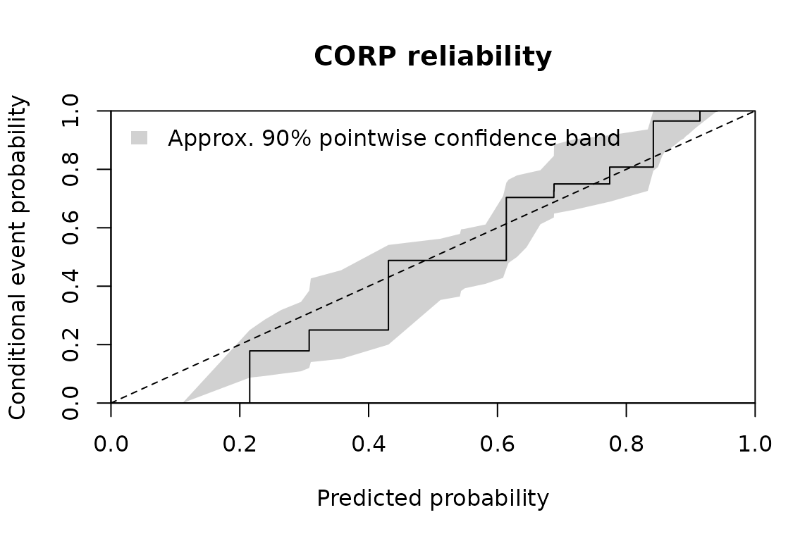

CORP reliability diagram with the approximate confidence band.

The cost grows with replicates times the number of pairs. For large assessment sets with many distinct probabilities, band = "none" skips the resampling.

CORP bands are not Venn-Abers bounds

The Venn-Abers values lower and upper of a prediction and the CORP band limits band_lower and band_upper answer different questions:

Venn-Abers bounds belong to one prediction. They come from the calibrator, need no outcome of that observation and are not confidence intervals.
CORP band limits belong to the assessment pairs. They are pointwise resampling quantiles at each distinct probability, not simultaneous over the curve, and they assume independent pairs.

A CORP band therefore says nothing about Venn-Abers validity, and a Venn-Abers width says nothing about calibration on assessment data. The returned columns are named apart for this reason.

Brier decomposition

corp_decomposition_plot() splits the Brier score of the same pairs into miscalibration (MCB), discrimination (DSC) and uncertainty (UNC), with brier = mcb - dsc + unc. Lower MCB and higher DSC are better; UNC depends on the outcomes only.

parts <- corp_decomposition_plot(assessment$truth, probability)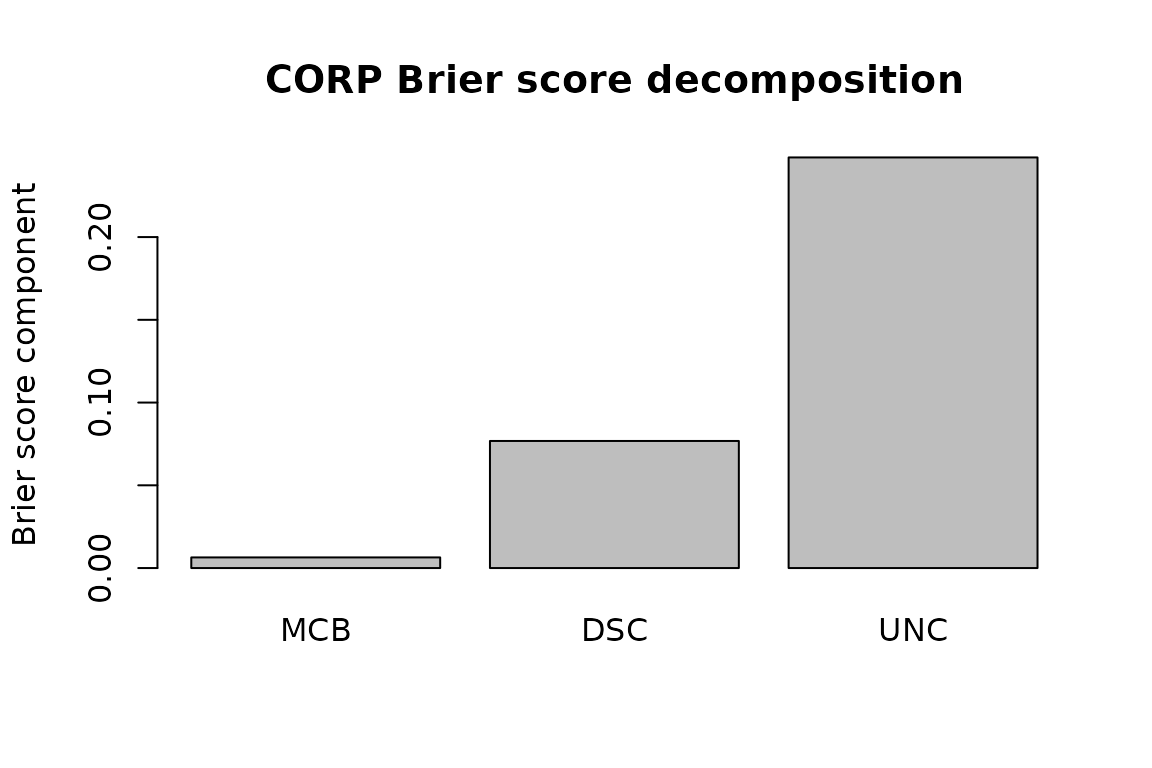

CORP decomposition of the Brier score.

parts
#>       brier         mcb        dsc       unc
#> 1 0.1777504 0.006425571 0.07679743 0.2481222
brier_score(assessment$truth, probability)
#> [1] 0.1777504

For factor truth, corp_plot() and corp_decomposition_plot() evaluate each class against the rest with its final probability, one panel or bar group per class. calibration_plot() remains available for binned reliability diagrams with a fixed number of equal-width bins.

Regression predictions

regression_plot() draws held-out observed values against the calibrated points, and with which = "residual" the residuals against the same points.

held_out <- 401:600
point <- predict(regression, uncalibrated[held_out])
held_out_pairs <- regression_plot(regression_data$truth[held_out],
                                  point$prediction,
                                  which = c("observed", "residual"))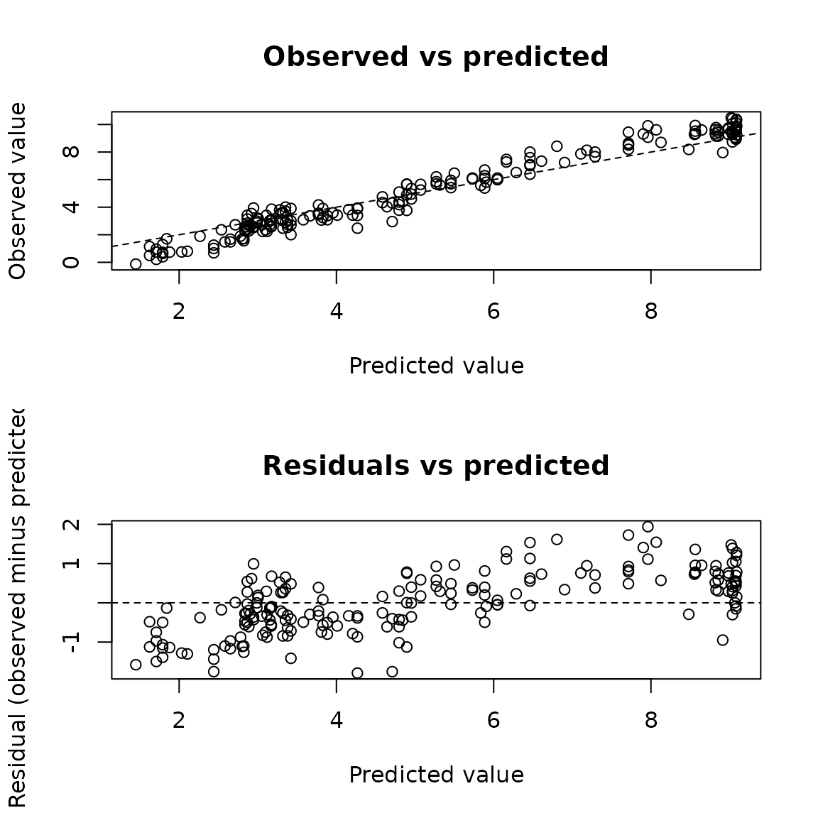

Observed values and residuals against calibrated regression points.

head(held_out_pairs)
#>   prediction    truth   residual
#> 1   5.456436 5.696566  0.2401304
#> 2   4.952644 4.595465 -0.3571795
#> 3   2.904895 2.623969 -0.2809264
#> 4   3.170868 2.588410 -0.5824581
#> 5   8.855605 9.432520  0.5769142
#> 6   5.070688 5.657558  0.5868698

It describes the pairs given and does not use the regression bounds lower and upper, which concern regularized conditional expectations, not the coverage of individual outcomes.