Assess Calibration with CORP Reliability Diagrams

Assesses the calibration of probabilities on evaluation pairs of truth and probability, held out from fitting the calibrator, such as an assessment set or a test set. Unlike plot.venn_abers, which shows the stored state of a fit, these graphics need new truth values.

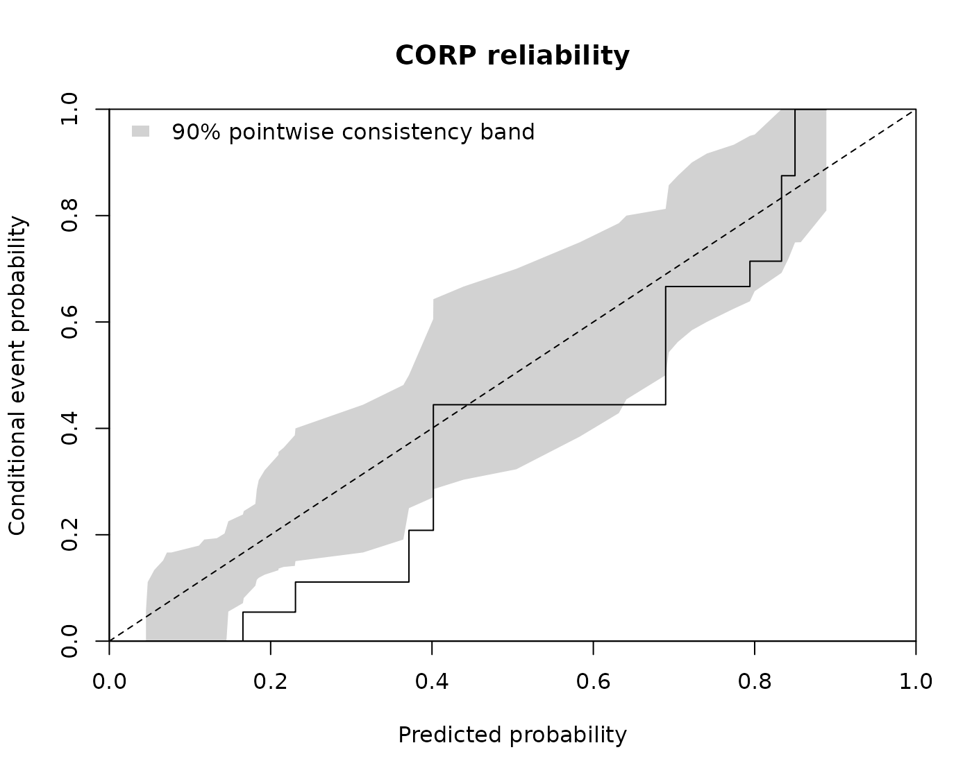
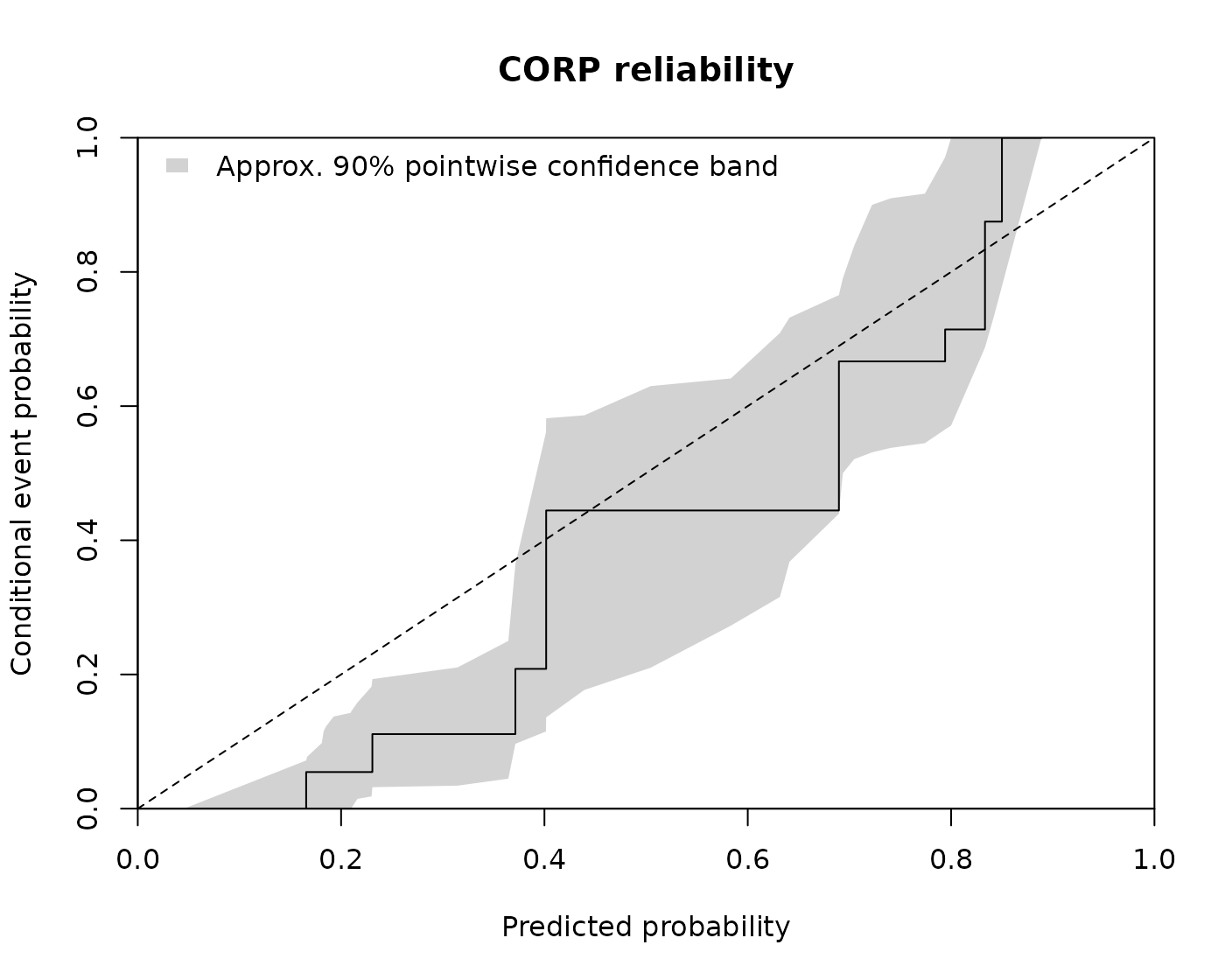
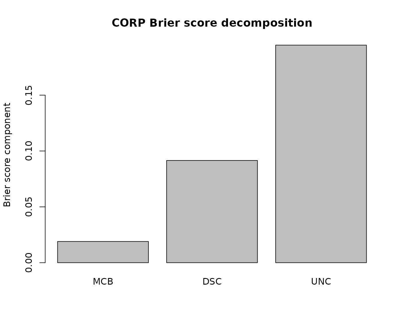
corp_plot() draws the CORP reliability diagram of Dimitriadis, Gneiting and Jordan (2021): the CORP estimate of the conditional event probability as a step over the probabilities, from the smallest to the largest, against the dashed diagonal of perfect calibration on [0, 1]. corp_decomposition_plot() draws the CORP decomposition of the Brier score as bars of miscalibration (MCB), discrimination (DSC), and uncertainty (UNC).

Usage

corp_plot(truth, probability, band = "consistency", level = 0.9,
          replicates = 1000, seed = NULL, ...)

corp_decomposition_plot(truth, probability, ...)

Arguments

truth: A non-empty logical or numeric vector containing only FALSE/0 and TRUE/1. TRUE/1 is the event class. Alternatively factor truth under the scoring contract in brier_score; assessment may omit observations of some levels.
probability: A numeric vector of regularized event probabilities, the same length as truth, with finite values in [0, 1]. For factor truth, the final class matrix under the input contract of venn_abers, never the internal pair probabilities.
band: Exactly one of "consistency" (default), "confidence", or "none": the uncertainty band drawn with the CORP estimate: the pointwise consistency band around the diagonal, the approximate pointwise confidence band around the estimate, or none. See the section on uncertainty bands.
level: One number strictly between 0 and 1: the pointwise level of the band.
replicates: One finite whole number of at least 1: the resampling replicates of the band. replicates * (1 - level) / 2 must be at least 1, so that each band quantile has a replicate beyond it.
seed: NULL or one integer in R's seed range for the band replicates. With a seed, the band is reproducible and the caller's random state is left unchanged; without one, the band draws from and advances the global random stream.
...: Base R graphical options passed to plot() in corp_plot() and to barplot() in corp_decomposition_plot(), taking precedence over the defaults in every panel.

Value

corp_plot() returns invisibly a data frame with one row per unique probability in increasing order and the same columns whatever band holds: probability, estimate (the CORP estimate of the conditional event probability), count (the pairs with this probability), band_lower and band_upper (the band limits), valid_replicates (the replicates defined at this probability, which the limits rest on), and the controls band, level, replicates, and seed, the same in every row. Without a band, band_lower, band_upper, and valid_replicates are NA, as they are when the confidence band is omitted; without a seed, seed is NA. The band limits are named apart from the Venn-Abers values lower and upper, which they are not.

corp_decomposition_plot() returns invisibly a data frame with one row and the columns brier, mcb, dsc, and unc.

For factor truth, both add a leading factor column class with the truth levels, grouping rows by class order.

Details

The CORP estimate is the isotonic (PAV) regression of the events on the probabilities, computed with isoreg. Equal probabilities are valid and pooled, so they share one estimate, and the estimate never decreases. Unlike the bins of calibration_plot, it needs no tuning.

With the PAV estimate q and the event rate r on the same pairs, mcb is the Brier score of the probabilities minus that of q, dsc the Brier score of r minus that of q, and unc the Brier score of r, so that brier = mcb - dsc + unc up to rounding. Lower mcb and higher dsc are better; unc depends on the truth only. The decomposition is deterministic.

Pairs are assumed independent. Both graphics describe the evaluation pairs given, conditional on the fitted calibrator; they make no statement about Venn-Abers validity.

Uncertainty bands

Both bands are computed by resampling as in the reliabilitydiag package (version 0.2.1). Each of the replicates draws the pairs with replacement, draws new events from the drawn probabilities themselves (consistency band) or from the CORP estimate at them (confidence band), fits PAV again with ties pooled, and interpolates that fit linearly at the unique probabilities, leaving it missing outside the drawn range. The band limits at each probability are the (1 - level) / 2 and (1 + level) / 2 quantiles of its valid replicates (quantile, type 7), so they lie in [0, 1] and equal probabilities share them. The band is drawn as a translucent gray area with a legend naming it; the limits are linearly interpolated between the unique probabilities.

The consistency band shows where the CORP estimate of a perfectly calibrated forecast with these probabilities would fall; an estimate outside it points to miscalibration there. It is a reference region, not a test of Venn-Abers validity. The confidence band resamples from the estimate itself and is only approximate: the bootstrap of an isotonic fit is not consistent for continuous probabilities, so the band claims no nominal coverage. It fares better with few distinct probabilities and many pairs at each, as Venn-Abers calibrators often produce. In a simulation study at level 0.9 with 1000 replicates, 1000 runs, and true conditional event probability x^2, its mean pointwise coverage at probabilities between 0.05 and 0.95 was 0.92 for 100 and 0.88 for 1000 uniform probabilities, and 0.95 and 0.91 for 100 and 1000 pairs on ten distinct probabilities. It varied along the curve, down to 0.34 just above 0.05 for 1000 uniform probabilities. The consistency band held the CORP estimate of calibrated probabilities with mean coverage between 0.90 and 0.93 in the same settings. At inner probabilities with an estimate of exactly 0 or 1, the confidence limits are interpolated linearly from the neighboring probabilities, a heuristic of the reference; at the smallest and largest probabilities the band stays narrow there. When the pairs (for factor truth, of a class) hold only one outcome, the confidence band is omitted with a warning and its limits are NA; the consistency band depends on the probabilities only and is always computed.

Both bands are pointwise at level for each probability, not simultaneous over the curve, and for factor truth they are computed class by class without joint coverage across classes. They assume independent pairs; dependent data such as time series or clusters need other methods. Small assessment sets give wide bands that say little. The band limits are not Venn-Abers lower and upper probabilities.

The cost grows with replicates times the number of pairs, each replicate sorting and fitting them again. The exact quantiles hold the replicate values at every unique probability in memory at once, a matrix of unique probabilities by replicates. With the default 1000 replicates and 100000 continuous probabilities, that matrix takes about 800 MB and the call about 2 GB at its peak, and one call takes minutes, the confidence band several times longer than the consistency band. Few distinct probabilities need far less. For large assessment sets, band = "none" skips the resampling.

Multiclass

Every factor, even with two levels, is evaluated class by class: each class against the rest, using its final probability. corp_plot() draws one panel per class, titled "CORP: <class>", in its own nearly square grid as in calibration_plot, and restores the previous graphical parameters on exit, also after errors. Its bands draw the replicates of the classes in turn from one random stream, set once by seed. corp_decomposition_plot() draws one panel of the components grouped side by side, one bar and legend entry per class, without a combined value.

Each brier is the binary Brier score of its class, mean((y_k - p_k)^2). Their sum over classes is the multiclass value of brier_score, which they do not replace.

References

Dimitriadis, T., Gneiting, T. and Jordan, A. I. (2021). Stable reliability diagrams for probabilistic classifiers. Proceedings of the National Academy of Sciences, 118(8), e2016191118. doi:10.1073/pnas.2016191118

Examples

set.seed(1)
score <- runif(400)
truth <- rbinom(400, 1, score^2)
fitting <- 1:200
calibrator <- venn_abers(truth[fitting], score[fitting])
assessment <- predict(calibrator, score[-fitting])$probability

corp_plot(truth[-fitting], assessment, seed = 1)

corp_plot(truth[-fitting], assessment, band = "confidence", replicates = 199, seed = 1)

corp_decomposition_plot(truth[-fitting], assessment)