Calibrating supplied predictions

vennabers calibrates predictions from an existing model. The manual functions use only base R and packages included with R: you train the model, supply its predictions and keep it for future use. For package-managed training and preprocessing, continue with vignette("workflows", package = "vennabers"). vignette("method", package = "vennabers") explains the methods and their guarantees.

Task	Inductive	Cross
Binary or multiclass classification	venn_abers()	cross_venn_abers()
Regression	venn_abers_regression()	cross_venn_abers_regression()

Inductive calibration uses one fixed model and a separate calibration set. Cross calibration fits a calibrator for each held-out fold and combines their results. Each fold’s model must exclude that fold from all learned steps, including preprocessing and tuning. That same retained model must supply its new-observation predictions. An all-data refit cannot replace these models in the manual Cross interface.

Final assessment data stay outside both training and calibration. If assessment results influence the choice of method or parameters, those rows become selection data and another untouched assessment set is needed. The examples below illustrate the interfaces; their small assessment sets are not benchmarks.

Binary Inductive calibration

Generate a reproducible binary example with a training, calibration and assessment set. Here TRUE is the event whose probability we calibrate.

library(vennabers)
set.seed(12)
data <- data.frame(x = rnorm(240))
data$truth <- runif(nrow(data)) < plogis(data$x)
training <- data[1:120, ]
calibration <- data[121:200, ]
assessment <- data[201:240, ]

model <- glm(truth ~ x, data = training, family = binomial())
calibration_p <- predict(model, calibration, type = "response")
new_p <- predict(model, assessment["x"], type = "response")
calibrator <- venn_abers(calibration$truth, calibration_p)
result <- predict(calibrator, new_p)
head(result)
#>       lower      upper probability
#> 1 0.0000000 0.09090909  0.08333333
#> 2 0.4642857 0.65217391  0.54901961
#> 3 0.7058824 0.76470588  0.72222222
#> 4 0.0000000 0.40000000  0.28571429
#> 5 0.3333333 0.50000000  0.42857143
#> 6 0.7058824 0.76470588  0.72222222

The result has lower, upper and probability columns in input row order. The endpoints are Venn-Abers bounds, not confidence intervals. The default log-loss regularization produces upper / (1 - lower + upper). Brier regularization uses upper + (lower^2 - upper^2) / 2 and can be selected at prediction time without refitting:

head(predict(calibrator, new_p, loss = "brier"))
#>       lower      upper probability
#> 1 0.0000000 0.09090909  0.08677686
#> 2 0.4642857 0.65217391  0.54728912
#> 3 0.7058824 0.76470588  0.72145329
#> 4 0.0000000 0.40000000  0.32000000
#> 5 0.3333333 0.50000000  0.43055556
#> 6 0.7058824 0.76470588  0.72145329
head(predict(calibrator, new_p, type = "class"))
#> [1] FALSE  TRUE  TRUE FALSE FALSE  TRUE

Binary classes are logical: an event probability of at least 0.5 gives TRUE. Use precision = 2 when fitting to round calibration probabilities to two decimal places. New probabilities remain unrounded. Changing precision needs a new calibrator; changing loss does not.

Score the regularized probabilities against the untouched assessment outcomes:

rbind(
  original = c(brier = brier_score(assessment$truth, new_p),
               log_loss = log_loss(assessment$truth, new_p)),
  calibrated = c(brier = brier_score(assessment$truth, result$probability),
                 log_loss = log_loss(assessment$truth, result$probability))
)
#>                brier  log_loss
#> original   0.1886682 0.5625150
#> calibrated 0.2122774 0.6182049

Lower is better for both scores. Calibration need not improve either score on a particular assessment set. A reliability diagram compares mean probability and observed event rate within bins; small bins can be noisy.

calibration_plot(assessment$truth, result$probability, bins = 5)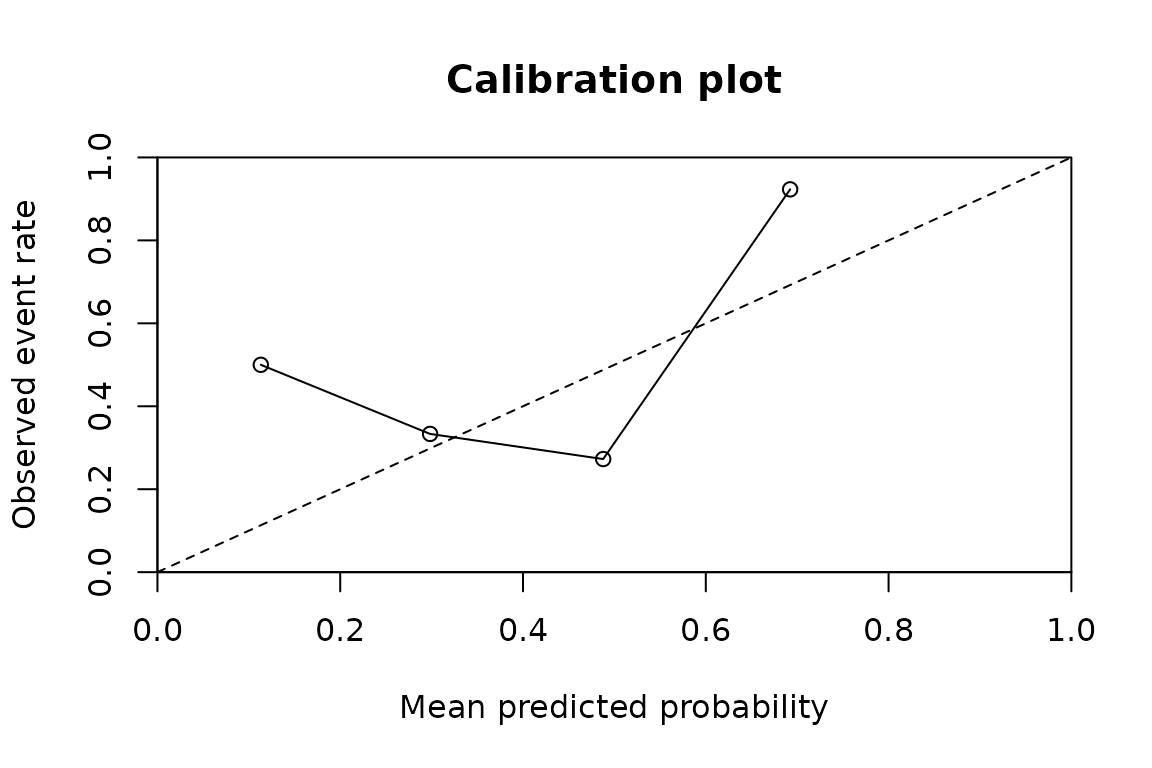

Calibration on the separate assessment set (five equal-width bins).

Fit diagnoses of the calibrator itself and CORP reliability diagrams with uncertainty bands are covered in vignette("diagnostics", package = "vennabers").

Binary Cross calibration: retain the fold models

Use the first 200 observations as development data, still keeping assessment separate. Each model below trains on the complement of its assigned fold.

development <- data[1:200, ]
set.seed(31)
fold <- sample(rep(c("A", "B", "C", "D"), length.out = nrow(development)))
models <- setNames(vector("list", 4), c("A", "B", "C", "D"))
oof_p <- numeric(nrow(development))
for (id in names(models)) {
  held <- fold == id
  models[[id]] <- glm(truth ~ x, data = development[!held, ],
                      family = binomial())
  oof_p[held] <- predict(models[[id]], development[held, ], type = "response")
}
cross <- cross_venn_abers(development$truth, oof_p, fold)

# Columns identify models; rows are the same new observations in every column.
fold_p <- vapply(models, predict, numeric(nrow(assessment)),
                 newdata = assessment["x"], type = "response")
head(predict(cross, fold_p))
#>   probability
#> 1   0.1440164
#> 2   0.5425838
#> 3   0.7705789
#> 4   0.2158523
#> 5   0.3175470
#> 6   0.7862010
cross_details <- predict(cross, fold_p, type = "details")
head(cross_details$folds)
#>   row fold     lower     upper probability
#> 1   1    A 0.0000000 0.1250000   0.1111111
#> 2   2    A 0.6333333 0.6666667   0.6451613
#> 3   3    A 0.6333333 0.6666667   0.6451613
#> 4   4    A 0.0000000 0.2000000   0.1666667
#> 5   5    A 0.0000000 0.5000000   0.3333333
#> 6   6    A 0.6333333 0.6666667   0.6451613

The input is a named matrix, one column per retained fold model. Columns match fold IDs by name; rows match by position. The default output contains only probability. There is no aggregate classification interval.

With log loss, Cross combines geometric means of the fold endpoints, rather than averaging fold point probabilities. With loss = "brier", it averages the Brier-regularized fold points. Both give each fold equal weight, even when fold sizes differ. type = "details" exposes the individual fold bounds and points. The Cross aggregate does not inherit the Inductive perfect-calibration guarantee; see ?predict.cross_venn_abers for the exact merger.

Multiclass: one-vs-one and one-vs-rest

Multiclass truth must be a factor. Probabilities must be a numeric matrix with columns named exactly after its levels, finite entries in [0, 1], and rows summing to one within 1e-8. Factor levels fix output order. Even a two-level factor selects this matrix interface; binary vector calibration instead uses logical or numeric 0/1 truth.

The following small, illustrative arrays stand in for predictions from a fixed model on separate calibration and assessment observations.

classes <- c("cat", "dog", "bird")
truth <- factor(rep(classes, 3), levels = classes)
p <- rbind(c(.7, .2, .1), c(.2, .6, .2), c(.1, .2, .7),
           c(.5, .3, .2), c(.3, .5, .2), c(.2, .3, .5),
           c(.6, .3, .1), c(.1, .7, .2), c(.2, .2, .6))
colnames(p) <- classes
new_p <- rbind(c(.6, .3, .1), c(.1, .4, .5), c(.2, .6, .2))
colnames(new_p) <- classes
new_truth <- factor(c("cat", "bird", "dog"), levels = classes)

One-vs-one (OvO) calibrates each class pair using only that pair’s rows, then couples the binary probabilities into one class vector. This does not train separate pairwise models. One-vs-rest (OvR) calibrates each class against all other classes using every row, then normalizes the class points.

ovo <- venn_abers(truth, p, method = "ovo")
ovr <- venn_abers(truth, p, method = "ovr")
predict(ovo, new_p)
#>            cat       dog      bird
#> [1,] 0.6162528 0.2370203 0.1467269
#> [2,] 0.1428571 0.4285714 0.4285714
#> [3,] 0.2000000 0.6000000 0.2000000
predict(ovr, new_p)
#>             cat       dog      bird
#> [1,] 0.62068966 0.2758621 0.1034483
#> [2,] 0.09677419 0.3870968 0.5161290
#> [3,] 0.15384615 0.6923077 0.1538462
predict(ovo, new_p, type = "class")
#> [1] cat dog dog
#> Levels: cat dog bird
head(predict(ovo, new_p, type = "details")$pairs)
#>   row non_event event     lower     upper probability
#> 1   1       cat   dog 0.0000000 0.3333333        0.25
#> 2   2       cat   dog 0.6666667 1.0000000        0.75
#> 3   3       cat   dog 0.6666667 1.0000000        0.75
#> 4   1       cat  bird 0.0000000 0.3333333        0.25
#> 5   2       cat  bird 0.6666667 1.0000000        0.75
#> 6   3       cat  bird 0.0000000 1.0000000        0.50
head(predict(ovr, new_p, type = "details")$classes)
#>   row event     lower     upper probability
#> 1   1   cat 0.6666667 1.0000000   0.7500000
#> 2   2   cat 0.0000000 0.1428571   0.1250000
#> 3   3   cat 0.0000000 0.2000000   0.1666667
#> 4   1   dog 0.0000000 0.5000000   0.3333333
#> 5   2   dog 0.0000000 1.0000000   0.5000000
#> 6   3   dog 0.6666667 1.0000000   0.7500000
c(brier = brier_score(new_truth, predict(ovo, new_p)),
  log_loss = log_loss(new_truth, predict(ovo, new_p)))
#>     brier  log_loss 
#> 0.3318605 0.6140738

Score the final class matrix, not pair diagnostics. Multiclass Brier scores sum squared errors across classes before averaging observations; their scale differs from the binary event-only score. Exact class ties select the first factor level. Diagnostic bounds describe binary subproblems, not multiclass confidence intervals. venn_abers_one_hot() turns class decisions into a 0/1 matrix with one column per class; the installed example one-hot-classes.R covers binary decisions, ties and missing values.

For manual Cross multiclass calibration, supply an out-of-fold class matrix and a shared fold vector. New predictions are a list of class matrices named by fold ID, with identical new-row order. This illustrative example assumes model A excluded the first six calibration rows and model B the last three:

multi_fold <- rep(c("A", "B"), c(6, 3))
fold_new <- list(A = new_p, B = (new_p + 1 / 3) / 2)
for (method in c("ovo", "ovr")) {
  fitted <- cross_venn_abers(truth, p, multi_fold, method = method)
  print(predict(fitted, fold_new))
}
#>            cat       dog      bird
#> [1,] 0.4185380 0.3377631 0.2436989
#> [2,] 0.2415253 0.3885493 0.3699254
#> [3,] 0.2679492 0.4641016 0.2679492
#>            cat       dog      bird
#> [1,] 0.4199778 0.3584735 0.2215488
#> [2,] 0.2215488 0.3584735 0.4199778
#> [3,] 0.2562838 0.4874323 0.2562838

Every class must occur globally; every OvO pair must have at least one row in each calibration fold. Merge folds within each pair or class first, then couple or normalize. Averaging already finished multiclass predictions is a different procedure.

Regression: moderated Inductive and Cross calibration

Regression accepts finite real-valued truth and predictions, including negative values. Train a numeric model on separate observations:

set.seed(52)
regression <- data.frame(x = rnorm(240))
regression$truth <- 2 * regression$x + rnorm(240, sd = .7)
reg_model <- lm(truth ~ x, data = regression[1:120, ])
reg_cal <- regression[121:200, ]
reg_test <- regression[201:240, ]
ivar <- venn_abers_regression(reg_cal$truth, predict(reg_model, reg_cal), m = 1)
reg_result <- predict(ivar, predict(reg_model, reg_test["x"]))
head(reg_result)
#>   prediction      lower      upper
#> 1  0.3488897  0.1058132  0.7791953
#> 2 -1.8819104 -3.0794773 -1.2437399
#> 3  1.4326392  1.1602332  2.8171219
#> 4 -0.6129800 -1.4915333  0.4290850
#> 5  1.8326324  1.6854866  3.5768573
#> 6 -0.6918746 -1.5179563  0.2347609
sqrt(mean((reg_test$truth - reg_result$prediction)^2))
#> [1] 1.137166

The result contains prediction, lower and upper in outcome units. The point uses a weighted merger of the bounds and is generally not their midpoint. For calibration size k, moderation must satisfy 1 <= m <= floor((k - 1) / 2); the default m = 1 needs at least three rows. Alternatively, supply only epsilon, which sets m = floor(epsilon * (k + 1) / 2) and must satisfy the same constraint. epsilon is a moderation parameter, not a prediction-interval error rate.

Cross regression uses the same model-to-fold matching as binary Cross:

reg_dev <- regression[1:200, ]
reg_models <- setNames(vector("list", 4), names(models))
oof_numeric <- numeric(nrow(reg_dev))
for (id in names(reg_models)) {
  held <- fold == id
  reg_models[[id]] <- lm(truth ~ x, data = reg_dev[!held, ])
  oof_numeric[held] <- predict(reg_models[[id]], reg_dev[held, ])
}
cvar <- cross_venn_abers_regression(reg_dev$truth, oof_numeric, fold, m = 1)
new_numeric <- vapply(reg_models, predict, numeric(nrow(reg_test)),
                      newdata = reg_test["x"])
reg_details <- predict(cvar, new_numeric, type = "details")
head(reg_details$prediction)
#>   prediction     lower       upper
#> 1  0.2595001 -0.362139  1.08649570
#> 2 -1.4972613 -2.671720 -0.99832704
#> 3  1.4058132  1.016085  3.10475672
#> 4 -0.5976522 -1.589646  0.29300056
#> 5  1.8034753  1.693239  4.01503281
#> 6 -0.7244145 -1.634716  0.02320936
head(reg_details$folds$A)
#>   prediction      lower      upper
#> 1  0.6792580  0.4568184  1.1479425
#> 2 -1.4882713 -2.4696040 -1.0289988
#> 3  1.5164484  1.3479463  2.7206618
#> 4 -0.4950529 -1.7157862  0.7805441
#> 5  1.7853971  1.7340951  3.3463712
#> 6 -0.7009826 -1.7304629  0.1784766

Every fold must support the requested moderation. CVAR averages complete fold points and each bound separately, with equal weights. It does not recompute a point from averaged bounds. Neither IVAR nor CVAR bounds are confidence or prediction intervals for future outcomes; Cross bounds are descriptive fold summaries and do not add a coverage guarantee.

Keeping the complete predictor

Save the calibrator and its matching model or models, for example saveRDS(list(models = models, calibrator = cross), "predictor.rds"). Load vennabers and the model’s required packages before predicting in a new session. The manual calibrator does not retain the underlying model.

The next vignette, vignette("workflows", package = "vennabers"), shows how to retain the complete preprocessing, model and calibration procedure together.

For the complete standalone scripts with a contents list, open vignette("examples-manual", package = "vennabers"). ?vennabers_examples indexes all four example collections.