vignette("method", package = "vennabers") describes how
Venn-Abers calibration relates to Platt scaling and isotonic
calibration. This guide puts the three side by side on one simulated
data set. It is a small illustration, not a benchmark: it shows what the
differences can look like, not which method is better in general. It
uses base R and the package only.
Data and their roles
The event probability is with a standard normal . The scoring model is a logistic regression that is linear in , so it is misspecified. Its scores increase with and rank cases correctly, but they are too extreme near and not extreme enough for large . The data have three roles, and each observation has exactly one:
- Training (500 observations) fits the scoring model.
- Calibration (300 observations) fits the three calibration maps from the model’s scores. The model never sees these observations.
- Assessment (2000 observations) scores the calibrated probabilities. No model and no calibration map sees them before.
Assessing on calibration observations would favor the most flexible map, because it has adapted to exactly these outcomes.
simulate <- function(event_probability, seed) {
  set.seed(seed)
  sizes <- c(training = 500, calibration = 300, assessment = 2000)
  x <- rnorm(sum(sizes))
  data <- data.frame(x = x, truth = runif(sum(sizes)) < event_probability(x))
  split(data, factor(rep(names(sizes), sizes), levels = names(sizes)))
}
data <- simulate(function(x) plogis(x^3), seed = 49)
sapply(data, nrow)
#>    training calibration  assessment
#>         500         300        2000
Three calibration maps
All three maps learn from the same calibration scores and outcomes and are applied to the same assessment scores:
-
Platt scaling fits a logistic regression of the
outcome on the logit of the score. This is maximum likelihood without
the smoothed targets that Platt
- proposes for small calibration sets.
-
Isotonic calibration (Zadrozny and Elkan, 2002)
fits a non-decreasing step function with
stats::isoreg(). A new score takes the value of the nearest calibration score below it, or of the lowest one if it lies below all of them. -
Venn-Abers calibration uses
venn_abers()and the default log-loss merger of its lower and upper values.
calibrate <- function(data) {
  model <- glm(truth ~ x, data = data$training, family = binomial())
  score <- predict(model, data$calibration, type = "response")
  new_score <- predict(model, data$assessment, type = "response")
  truth <- data$calibration$truth

  platt <- glm(truth ~ qlogis(score), family = binomial())
  platt_probability <- plogis(coef(platt)[[1]] +
                                coef(platt)[[2]] * qlogis(new_score))

  o <- order(score)
  isotonic <- stats::isoreg(score[o], truth[o])
  isotonic_map <- stats::approxfun(score[o], isotonic$yf, method = "constant",
                                   rule = 2, ties = mean)

  venn_abers_probability <- predict(venn_abers(truth, score),
                                    new_score)$probability

  list(truth = data$assessment$truth,
       probability = list(Uncalibrated = new_score,
                          Platt = platt_probability,
                          Isotonic = isotonic_map(new_score),
                          `Venn-Abers` = venn_abers_probability))
}
result <- calibrate(data)
Results
The table scores each method on the assessment set. Lower log loss and lower Brier score are better. The last column counts assessment probabilities of exactly 0 or 1.
score_methods <- function(result) {
  t(sapply(result$probability, function(probability) {
    c(log_loss = log_loss(result$truth, probability),
      brier_score = brier_score(result$truth, probability),
      at_0_or_1 = sum(probability %in% c(0, 1)))
  }))
}
scores <- score_methods(result)
knitr::kable(scores, digits = 4)| log_loss | brier_score | at_0_or_1 | |
|---|---|---|---|
| Uncalibrated | 0.5719 | 0.1974 | 0 |
| Platt | 0.5702 | 0.1976 | 0 |
| Isotonic | Inf | 0.1929 | 356 |
| Venn-Abers | 0.5557 | 0.1927 | 0 |
The CORP reliability diagrams of corp_plot() show the
same probabilities against the event frequencies estimated from the
assessment outcomes. A well calibrated method follows the diagonal; the
gray band shows where the curve of perfectly calibrated probabilities
would fall by chance.
old <- par(mfrow = c(2, 2))
for (method in names(result$probability)) {
  corp_plot(result$truth, result$probability[[method]], seed = 1, main = method)
}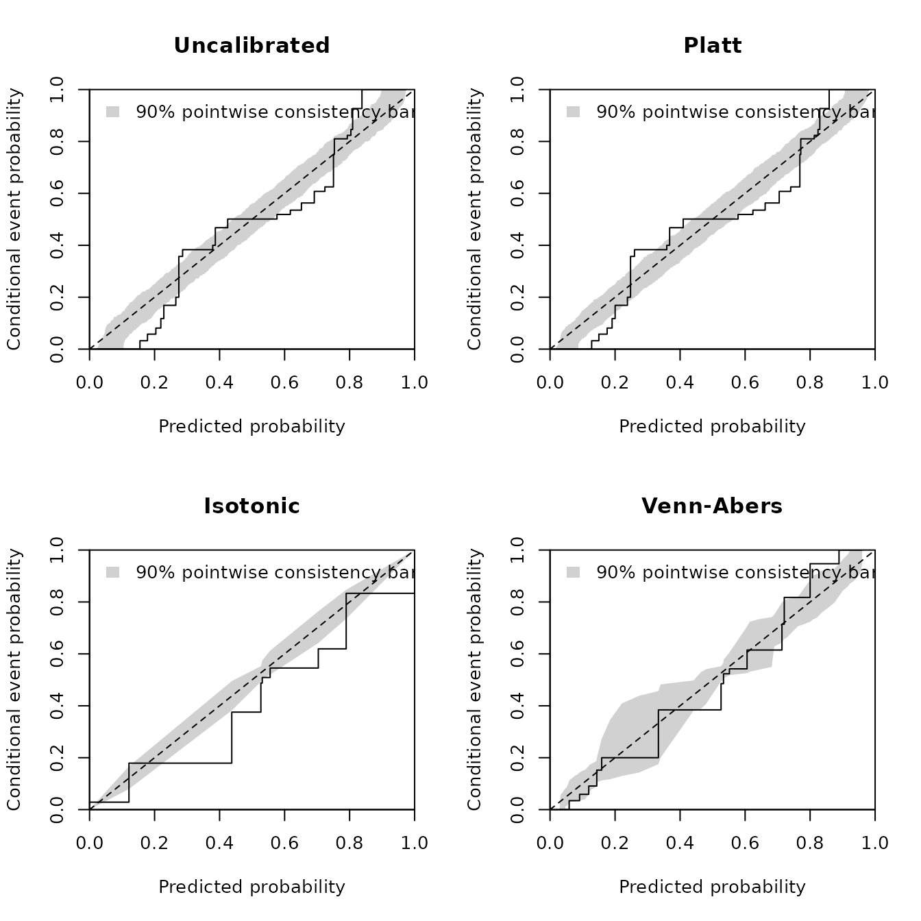
CORP reliability diagrams on the assessment set.
par(old)Isotonic calibration uses only 9 distinct probabilities, and some cases that it sets to exactly 0 or 1 have the other outcome:
isotonic <- result$probability$Isotonic
extreme <- isotonic %in% c(0, 1)
table(probability = isotonic[extreme], event = result$truth[extreme])
#>            event
#> probability FALSE TRUE
#>           0   203    6
#>           1     3  144
On this data set:
- The uncalibrated model is visibly miscalibrated. Its curve crosses the diagonal several times and leaves the band, as expected from scores that are too extreme near 0.5 and not extreme enough near 0 and 1.
- Platt scaling hardly changes it. The logit of a logistic model’s score is linear in , so a logistic map of it is still a logistic function of and cannot represent . Its log loss is 0.5702 against 0.5719 without calibration, and its Brier score is no better.
- Isotonic calibration removes most of the systematic pattern and has a low Brier score. Its few steps, learned from 300 observations, are off in places, and every case at 0 or 1 with the other outcome makes the log loss infinite.
- Venn-Abers calibration also removes the pattern, and its curve stays close to the diagonal. Its probabilities never reach 0 or 1. It has the lowest log loss of the four (0.5557), and its Brier score is close to the isotonic one.
A contrast: a well-specified model
The ranking depends on the data. If the event probability is itself logistic in , here , the scoring model is correctly specified. Its miscalibration is then only estimation error of a sigmoid shape, which Platt scaling models with two parameters. The flexible maps spend 300 calibration observations on a shape that needs no correction.
contrast <- score_methods(calibrate(simulate(function(x) plogis(0.3 + 1.5 * x),
                                             seed = 49)))
knitr::kable(contrast, digits = 4)| log_loss | brier_score | at_0_or_1 | |
|---|---|---|---|
| Uncalibrated | 0.5488 | 0.1841 | 0 |
| Platt | 0.5462 | 0.1827 | 0 |
| Isotonic | Inf | 0.1866 | 318 |
| Venn-Abers | 0.5516 | 0.1851 | 0 |
Platt scaling now has the lowest log loss and Brier score. Venn-Abers calibration does slightly worse than the uncalibrated model, and isotonic calibration again reaches 0 or 1.
What this does and does not show
The example shows mechanisms that the method guide describes: Platt scaling cannot correct a miscalibration that is not sigmoid-shaped, isotonic calibration can output 0 or 1 and then have an infinite log loss, and the Venn-Abers merger avoids both. It does not show more:
- One data set. Both settings are simulated with one seed, one scoring model and fixed set sizes. Another seed or other sizes can reorder methods whose scores are close, such as isotonic and Venn-Abers calibration in Brier score.
- No general superiority. Which method does best depends on the shape of the miscalibration and on the size of the calibration set. For an empirical comparison on several data sets, see Vovk, Petej and Fedorova (2015, Section 6).
-
No guarantee is tested. The validity guarantee of
Venn-Abers predictors concerns the pair of lower and upper values over
repeated data sets, not the merged probability on one assessment set;
see
vignette("method", package = "vennabers"). - Scores are not uncertainty. The table has no standard errors. With 2000 assessment observations, small differences can be noise.
vignette("diagnostics", package = "vennabers") explains
the CORP diagrams and the other assessment tools used here.
References
Dimitriadis, T., Gneiting, T. and Jordan, A. I. (2021). Stable reliability diagrams for probabilistic classifiers. Proceedings of the National Academy of Sciences, 118(8), e2016191118. doi:10.1073/pnas.2016191118
Platt, J. C. (2000). Probabilities for SV machines. In A. J. Smola, P. L. Bartlett, B. Schölkopf and D. Schuurmans (Eds.), Advances in Large Margin Classifiers, 61–74. MIT Press.
Vovk, V., Petej, I. and Fedorova, V. (2015). Large-scale probabilistic predictors with and without guarantees of validity. Advances in Neural Information Processing Systems 28, 892–900. doi:10.48550/arXiv.1511.00213
Zadrozny, B. and Elkan, C. (2002). Transforming classifier scores into accurate multiclass probability estimates. Proceedings of the Eighth ACM SIGKDD International Conference on Knowledge Discovery and Data Mining, 694–699. doi:10.1145/775047.775151