Assess Regression Predictions on Held-Out Pairs

Assesses regression predictions on evaluation pairs of truth and prediction, held out from fitting the calibrator, such as an assessment set or a test set. Unlike plot.venn_abers_regression, which shows the stored state of a fit, this graphic needs new truth values.

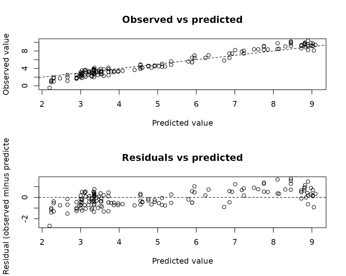
which = "observed" draws the observed against the predicted values with the dashed diagonal of equality, titled "Observed vs predicted". which = "residual" draws the residuals, observed minus predicted, against the predicted values with a dashed horizontal line at zero, titled "Residuals vs predicted".

Usage

regression_plot(truth, prediction, which = "observed", ...)

Arguments

truth

A non-empty numeric vector of finite observed values.

prediction

A numeric vector of finite predicted values, the same length as truth, such as the prediction column of predict.venn_abers_regression.

which

One or more distinct values of "observed" (default) and "residual": the diagrams to draw.

...

Base R graphical options passed to plot(), taking precedence over the defaults in every panel.

Value

Invisibly, a data frame with one row per pair in input order and the columns prediction, truth, and residual (truth - prediction), the same whatever which holds.

Details

The pairs are drawn as points, without a smoother. Choosing both diagrams draws them in this order, one above the other over the same predictions, in their own grid, and restores the previous graphical parameters on exit, also after errors.

Invalid pairs are errors; there is no na.rm. The graphic describes the evaluation pairs given and makes no statement about the Venn-Abers regression bounds lower and upper, which it does not use.

See also

venn_abers_regression for regression calibrators, plot.venn_abers_regression for their fit diagnoses, and corp_plot and calibration_plot for held-out classification probabilities. vignette("diagnostics", package = "vennabers") compares both kinds of graphics.

Examples

set.seed(1)
score <- runif(300, 0, 10)
truth <- score + sin(score) + rnorm(300, sd = .5)
fitting <- 1:150
calibrator <- venn_abers_regression(truth[fitting], score[fitting])
assessment <- predict(calibrator, score[-fitting])$prediction

regression_plot(truth[-fitting], assessment)
regression_plot(truth[-fitting], assessment, which = c("observed", "residual"))