Plot the Calibration Map of a Fitted Venn-Abers Calibrator

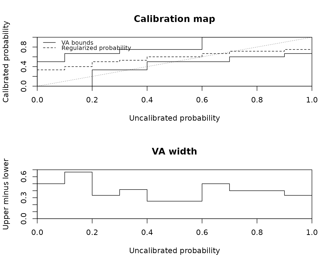
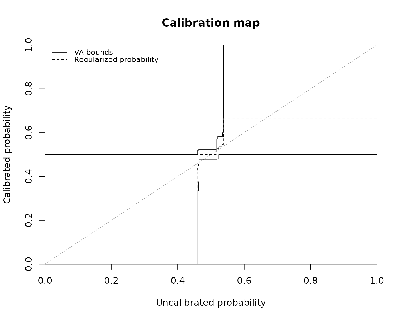
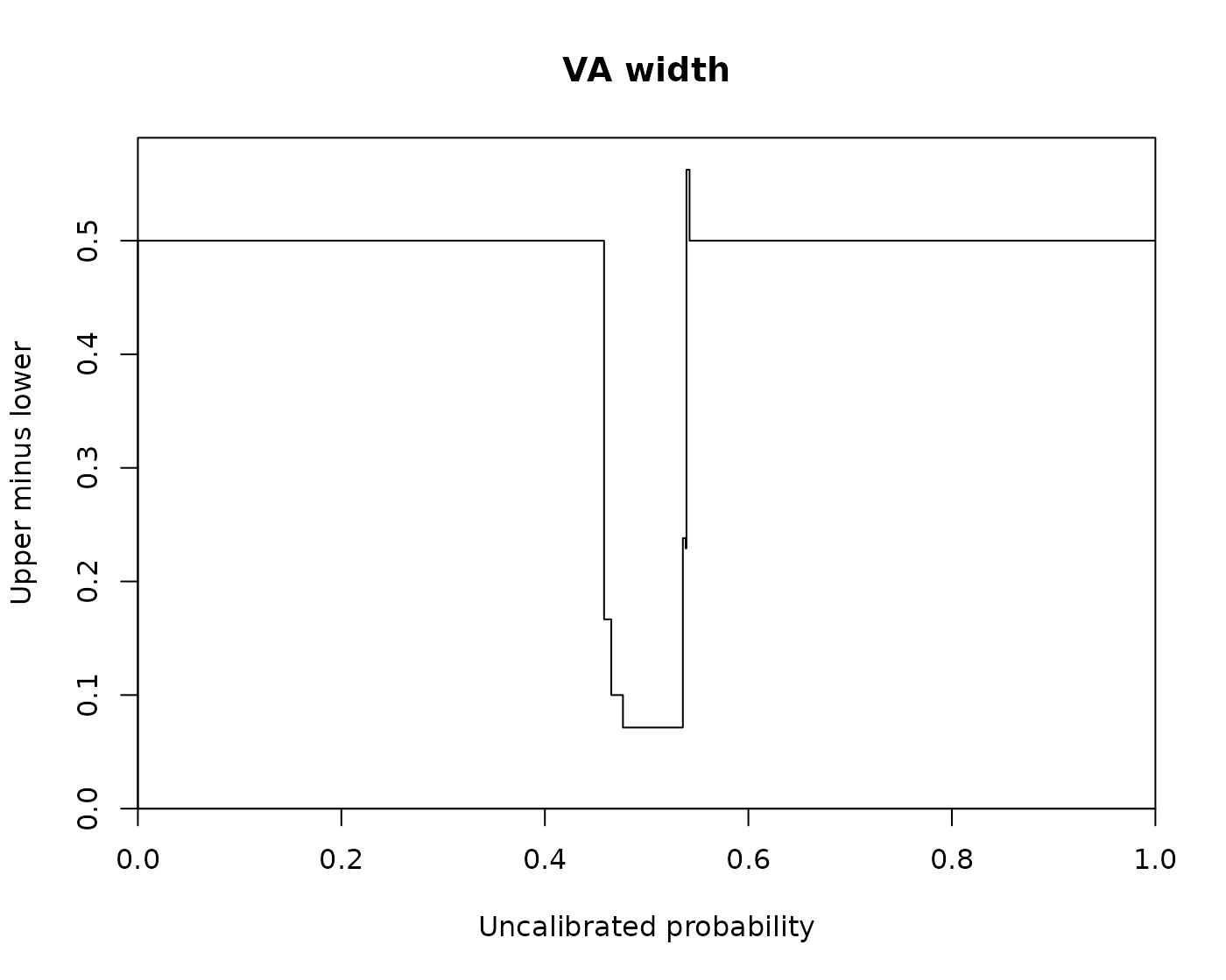
Draws a fit diagnosis from the stored state of a fitted calibrator, without new truth values. For classification, the calibration map shows the lower and upper Venn-Abers values as steps and the regularized probability as a dashed line over the uncalibrated probability on [0, 1]. The width diagram shows upper - lower over the same scores; it is neither a confidence level nor a nominal coverage.

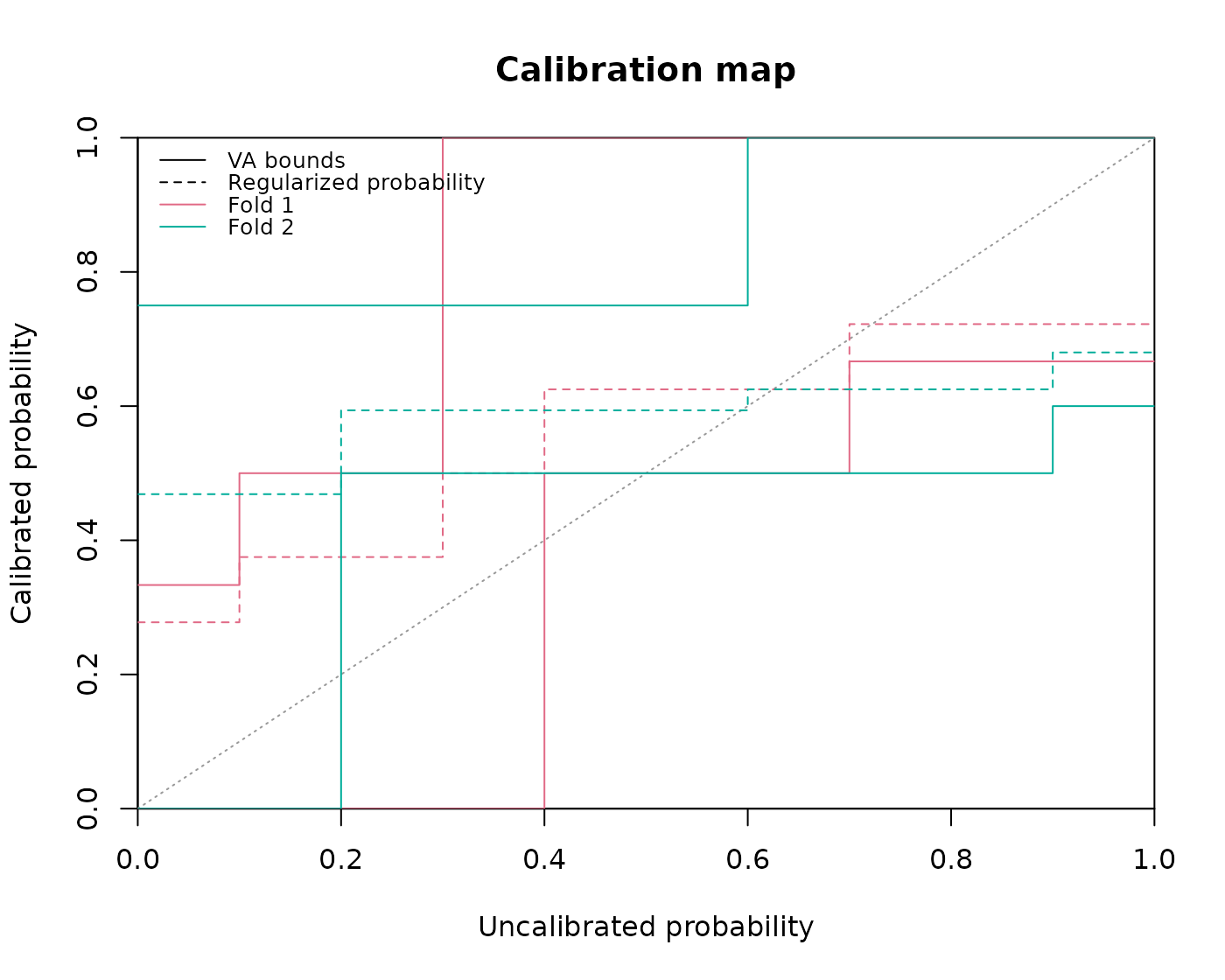
Cross fits overlay the map of every fold calibrator in one panel, distinguished by color and legend. Comparing fold maps at common scores does not describe the spread of an individual Cross prediction.

Choosing both diagrams draws them in their own grid of panels and restores the previous graphical parameters on exit, also after errors. A single diagram uses the current layout. Fits without a stored calibration map (knots, lower, upper) are errors; refit them with vennabers 1.0.0.

Usage

# S3 method for class 'venn_abers'
plot(x, which = "map", loss = "log", ...)

# S3 method for class 'cross_venn_abers'
plot(x, which = "map", loss = "log", ...)

# S3 method for class 'venn_abers_regression'
plot(x, which = "map", ...)

# S3 method for class 'cross_venn_abers_regression'
plot(x, which = "map", ...)

# S3 method for class 'vennabers_fit'
plot(x, which = "map", loss = x$loss, ...)

Arguments

x: A fitted binary or multiclass venn_abers or cross_venn_abers object, or a fitted venn_abers_regression or cross_venn_abers_regression object. For plot.vennabers_fit, a frozen fit from calibrate_workflow or the engine fit of a trained calibrated_workflow, extracted with workflows::extract_fit_engine(); see the Workflows section.
which: A character vector of distinct diagrams from "map" (default), the calibration map, and "width", the Venn-Abers width upper - lower. Both draw the map before the width, whatever their order.
loss: Exactly "log" (default) or "brier": the regularization of the drawn and returned probability, as in predict.venn_abers. Classification only: regression methods take no loss, and passing one is an error. For a workflow fit, the default is the loss stored at fitting.
...: Base R graphical options passed to plot(), taking precedence over the defaults in every panel. For regression, xlim also sets the range of the returned table.

Value

Invisibly, a data frame with the same columns whatever which holds: score, lower, upper, probability, and width. Rows hold each stored probability knot plus the range ends 0 and 1 in increasing order. Values are those of predict() at score with the chosen loss, and width is upper - lower.

For cross_venn_abers, a leading character column fold holds the stored fold IDs. Rows group by fold in stored order, each with its own knots and the values of its own fold calibrator, not the aggregated Cross probability.

For multiclass fits, the tables of all subproblems are stacked in stored order, with identity columns named as in venn_abers_details after fold and before the values: class for one-vs-rest, class_1 and class_2 for one-vs-one. Within a Cross subproblem, folds follow the stored fold IDs of the fit.

For regression, the columns are score, lower, upper, prediction, and width, after fold for cross_venn_abers_regression, with the values of predict() at score. The range ends replace 0 and 1; see the Regression section.

For a workflow fit, the table is that of its stored Venn-Abers calibrator. A pairwise fit stacks the tables of its pair components in stored order, led by the identity columns pair_id, then fold for Cross fits, then class_1 and class_2, as in venn_abers_details.

Between neighboring rows, the map holds the lower value of the left row and the upper value of the right row, so the width between knots exceeds the width at them. The drawn curves follow these values exactly.

Multiclass

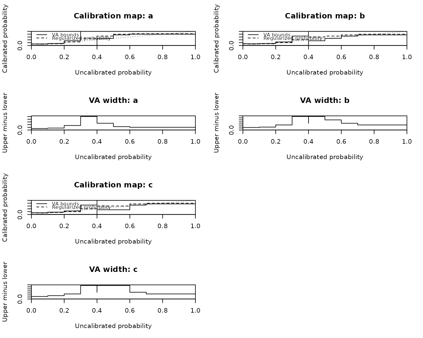
A multiclass fit draws one panel per subproblem and diagram, titled "Calibration map: <class>" for one-vs-rest and "Calibration map: <class_1> vs <class_2>" for one-vs-one (likewise "VA width"). Each panel shows the map of the subproblem's own binary calibrator over its score: the probability of the class for one-vs-rest, and the probability of class_2 renormalized within the pair for one-vs-one. The final coupling into class probabilities is not drawn. Cross fits overlay the fold maps of each subproblem in its panel, each fold in the same color across panels.

The panels fill their own grid row by row, nearly square as in calibration_plot. With both diagrams, each row of maps is followed by the widths of the same subproblems. A single panel, as for one one-vs-one pair, uses the current layout. Options in ... apply to every panel.

Regression

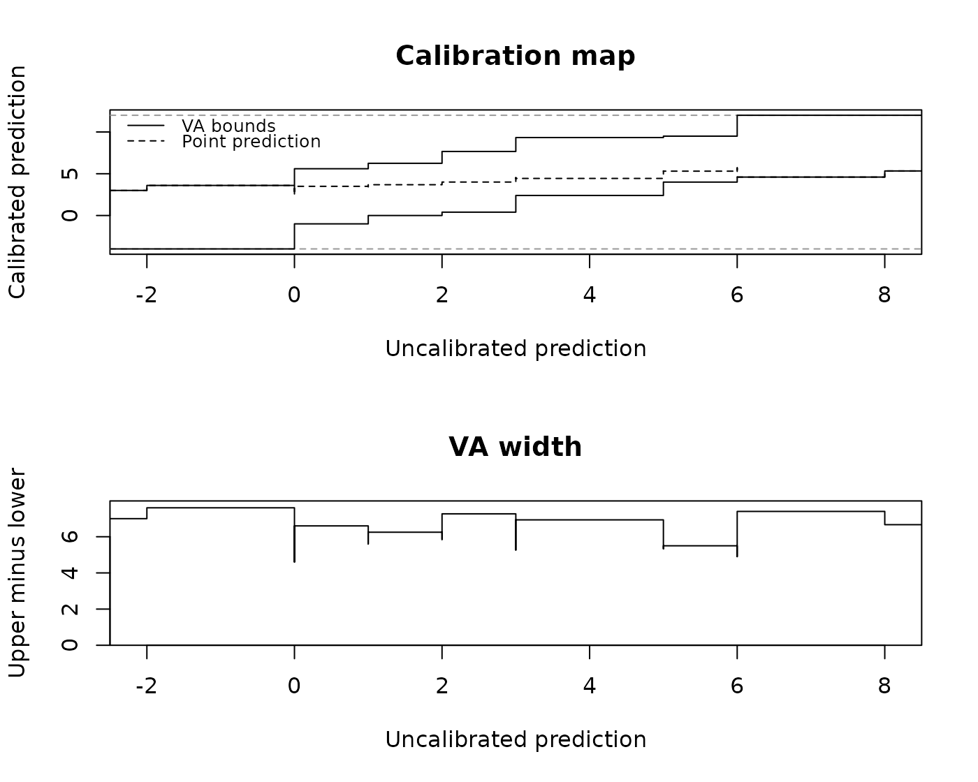
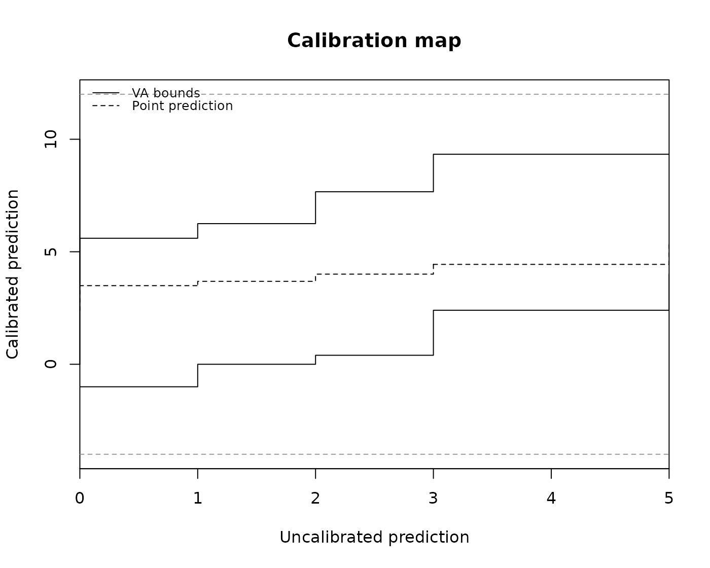
A regression fit draws the lower and upper Venn-Abers values as steps and the point prediction as a dashed line over the uncalibrated prediction, with gray dashed reference lines at the moderated truth values a and b that bound every Venn-Abers value. The width diagram shows upper - lower in units of the outcome.

The drawn range spans the stored knots, widened on each side by 5 % of their span; a single knot widens by 5 % of its absolute value, or 0.05 at zero. A Cross fit spans the knots of all folds, overlays its fold maps with a reference line at each fold's a and b, and returns every fold map over this shared range. A finite xlim in ... replaces the range: the table then holds its ends and the knots within.

Workflows

plot() on a frozen fit from calibrate_workflow, and on workflows::extract_fit_engine(fit) for a trained calibrated_workflow, draws the fit diagnosis of the stored Venn-Abers calibrator: binary, multiclass, or regression, inductive or Cross, as described above for that calibrator, with the same table. There is no method for the workflow itself. Postprocessing models (sigmoid, tailor, isotonic, or their ensembles) are source models before the calibrator: the map shows the calibrator over their output, not the postprocessing step.

A pairwise fit (model_training = "pairwise") draws one panel per pair component and diagram, titled "Calibration map: <class_1> vs <class_2>", in a grid as for multiclass fits. Each panel shows the binary calibrator of its pair over the probability of class_2 from that pair's own model.

A fit without a stored Venn-Abers calibrator is an error.

Examples

truth <- c(FALSE, TRUE, FALSE, TRUE, TRUE, FALSE, TRUE, TRUE)
uncalibrated_probability <- c(0.1, 0.2, 0.3, 0.4, 0.4, 0.6, 0.7, 0.9)
calibrator <- venn_abers(truth, uncalibrated_probability)

map <- plot(calibrator, which = c("map", "width"))

head(map)
#>   score     lower     upper probability     width
#> 1   0.0 0.0000000 0.5000000   0.3333333 0.5000000
#> 2   0.1 0.0000000 0.5000000   0.3333333 0.5000000
#> 3   0.2 0.3333333 0.6666667   0.5000000 0.3333333
#> 4   0.3 0.3333333 0.6666667   0.5000000 0.3333333
#> 5   0.4 0.5000000 0.7500000   0.6000000 0.2500000
#> 6   0.6 0.5000000 0.7500000   0.6000000 0.2500000

cross <- cross_venn_abers(truth, uncalibrated_probability, fold = rep(1:2, 4))
plot(cross, loss = "brier")


classes <- c("a", "b", "c")
class_truth <- factor(rep(classes, 4), levels = classes)
class_probability <- prop.table(matrix(c(
  6, 3, 1, 2, 5, 3, 1, 2, 7, 5, 1, 4, 3, 4, 3, 2, 2, 6,
  4, 4, 2, 1, 6, 3, 3, 3, 4, 5, 3, 2, 2, 7, 1, 2, 2, 6
), 12, 3, byrow = TRUE, dimnames = list(NULL, classes)), 1)
ovr <- venn_abers(class_truth, class_probability, method = "ovr")
head(plot(ovr, which = c("map", "width")))

#>   class score lower     upper probability     width
#> 1     a   0.0   0.0 0.1111111   0.1000000 0.1111111
#> 2     a   0.1   0.0 0.1111111   0.1000000 0.1111111
#> 3     a   0.2   0.0 0.1428571   0.1250000 0.1428571
#> 4     a   0.2   0.0 0.2500000   0.2000000 0.2500000
#> 5     a   0.3   0.0 0.3333333   0.2500000 0.3333333
#> 6     a   0.4   0.5 1.0000000   0.6666667 0.5000000

outcome <- c(-4, 1, 0, 3, 2, 6, 5, 9, 7, 12)
uncalibrated_prediction <- c(-2, 0, 0, 1, 2, 3, 3, 5, 6, 8)
regression <- venn_abers_regression(outcome, uncalibrated_prediction)
head(plot(regression, which = c("map", "width")))

#>   score lower    upper prediction    width
#> 1  -2.5  -4.0 3.000000   3.000000 7.000000
#> 2  -2.0  -4.0 3.000000   3.000000 7.000000
#> 3   0.0  -1.0 3.600000   2.389474 4.600000
#> 4   1.0   0.0 5.600000   3.446154 5.600000
#> 5   2.0   0.4 6.250000   3.714039 5.850000
#> 6   3.0   2.4 7.666667   4.526294 5.266667
plot(regression, xlim = c(0, 5))

if (all(vapply(c("parsnip", "workflows", "hardhat", "rsample", "recipes",
                "rlang", "tibble", "withr", "generics", "tidyselect"),
               requireNamespace, logical(1), quietly = TRUE))) {
  d <- data.frame(x = sin(1:80), truth = factor(rep(c("yes", "no", "no", "yes"), 20)))
  base <- workflows::workflow() |>
    workflows::add_formula(truth ~ x) |>
    workflows::add_model(parsnip::logistic_reg(engine = "glm"))
  frozen <- calibrate_workflow(generics::fit(base, d[1:40, ]), d[41:80, ], "truth")
  print(head(plot(frozen)))

  trained <- generics::fit(calibrated_workflow(base, "truth", seed = 42), d)
  plot(workflows::extract_fit_engine(trained), which = "width")
}

#>       score     lower upper probability     width
#> 1 0.0000000 0.0000000   0.5   0.3333333 0.5000000
#> 2 0.4584661 0.3333333   0.5   0.4285714 0.1666667
#> 3 0.4586977 0.3333333   0.5   0.4285714 0.1666667
#> 4 0.4590429 0.3333333   0.5   0.4285714 0.1666667
#> 5 0.4597943 0.3333333   0.5   0.4285714 0.1666667
#> 6 0.4602826 0.3333333   0.5   0.4285714 0.1666667