Note
This page was generated from the notebook examples/06_profile_likelihood.ipynb.
Profile-likelihood CIs — Wald vs. profile vs. sandwich#
The default confint(level=0.95) on a tram fit returns the Wald interval
where \(V = \text{vcov}() = -H^{-1}\) is the inverse observed information. Two assumptions are baked in: the log-likelihood is locally a well-conditioned paraboloid around \(\hat\theta\), and that paraboloid is symmetric. Both can fail — most visibly when the MLE sits on (or near) an active monotonicity boundary, which is the typical situation for the Bernstein coefficients of a small-\(n\) baseline transformation.
mltpy 0.4 exposes two non-Wald alternatives on the same confint() method (type="profile") and sandwich_se() helper:
Profile likelihood —
confint(type="profile")inverts the \(\chi^2_1\) likelihood-ratio test by re-fitting the constrained model with \(\theta_j\) pinned to a sweep of values and root-finding for \(2\,(\hat\ell - \ell_p(v)) = \chi^2_{1,1-\alpha}\). Honours likelihood asymmetry; pays roughly ten constrained refits per parameter.Sandwich —
sandwich_se()returns the HC0 estimator \(V_{\text{sand}} = B\,M\,B\) with \(B = -H^{-1}\) and \(M = \sum_i s_i s_i^\top\), robust to mild mis-specification of the outcome distribution. We assemble the symmetric CI manually as \(\hat\theta_j \pm z_{1-\alpha/2}\sqrt{V_{\text{sand},jj}}\).
This vignette compares all three on the right-censored Coxph fixture from reference/vcov_coxph_* — the same dataset that the R-parity tests in tests/test_confidence.py check element-wise against tram::Coxph(Surv(y, event) ~ x). The Bernstein MLE has Bs1 = Bs2 = Bs3 stacked on the monotonicity boundary, so the Wald approximation breaks down on those baseline coefficients while the well-identified covariate \(\beta_x\) remains a regular-asymptotics story where all three agree.
Below we render two figures: a forest plot of the three intervals side-by-side, then the profile log-likelihood curve for the most asymmetric parameter with all CI endpoints annotated.
[1]:
import warnings
from pathlib import Path

import matplotlib.pyplot as plt
import numpy as np
import pandas as pd
from scipy.stats import chi2, norm

from mltpy.model import ConvergenceWarning
from mltpy.tram import Coxph
from mltpy.variables import CensoredData

# Profile-CI refits a constrained likelihood ~10× per parameter; the inner
# auglag occasionally hits the outer-iteration cap on Bernstein-boundary
# pins and emits ConvergenceWarning (see CLAUDE.md, _PROFILE_INNER_KKT_THRESHOLD).
# The vignette is informational, not a parity test, so we silence them.
warnings.filterwarnings("ignore", category=ConvergenceWarning)

plt.rcParams["figure.dpi"] = 110
REF_DIR = Path("../../reference")  # repo-relative path to reference fixtures
1. The fitted model#
Right-censored Coxph fit on \(n = 200\) observations with one continuous covariate. Loading the dataset from reference/ rather than re-synthesising means the CI tables below are the same numbers the R-parity tests check against — tram::Coxph agrees to ~1e-3 on every row of both confint(type='wald') and confint(type='profile').
[2]:
y = np.loadtxt(REF_DIR / "vcov_coxph_y.txt")
x = np.loadtxt(REF_DIR / "vcov_coxph_x.txt").reshape(-1, 1)
event = np.loadtxt(REF_DIR / "vcov_coxph_event.txt").astype(int)
a, b = (float(v) for v in np.loadtxt(REF_DIR / "vcov_coxph_support.txt"))

cd = CensoredData.right_censored(y, censored=event == 0)
model = Coxph(support=(a, b), order=4).fit(cd, X=x)

param_names = [f"Bs{i}" for i in range(5)] + ["x"]
ll_hat = model.score(cd, X=x)

print(f"n = {len(y)}, events = {int(event.sum())}, censored = {(event == 0).sum()}")
print(f"log-likelihood at MLE = {ll_hat:.4f}")
print("theta_hat:")
for name, th in zip(param_names, model.theta_):
    print(f"  {name:>4} = {th:+.4f}")
n = 200, events = 147, censored = 53
log-likelihood at MLE = -168.1675
theta_hat:
   Bs0 = -2.4380
   Bs1 = +1.1091
   Bs2 = +1.1091
   Bs3 = +1.1091
   Bs4 = +1.8148
     x = +0.2383
Notice Bs1 = Bs2 = Bs3 ≈ 1.109 — three consecutive Bernstein coefficients have collapsed onto the monotonicity boundary \(\theta_{k+1} \ge \theta_k\). Equality-active constraints make the observed information singular along the boundary direction, and the Wald CI is the diagnostic that catches it most loudly.
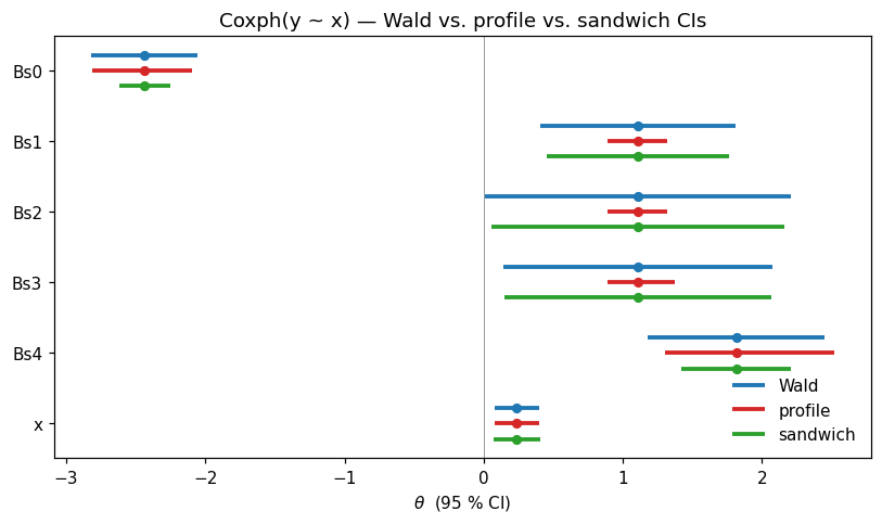
2. Wald, profile, and sandwich side-by-side#
All three share confint’s coverage target (95 %) and the same \(\hat\theta\). They differ only in how they convert the local likelihood geometry into an interval:
Wald —
confint(type="wald"): symmetric, uses \(\sqrt{V_{jj}} = \sqrt{(-H^{-1})_{jj}}\).Profile —
confint(type="profile"): inverts the LR test, asymmetric in general.Sandwich — assembled by hand as \(\hat\theta_j \pm z_{0.975}\,\sqrt{V_{\text{sand},jj}}\) using
sandwich_se(). Still symmetric; the only thing it replaces is the variance estimator.
[3]:
ci_wald = model.confint(level=0.95, type="wald")
ci_prof = model.confint(level=0.95, type="profile")
se_sand = model.sandwich_se()
z = float(norm.ppf(0.975))
ci_sand = np.column_stack((model.theta_ - z * se_sand, model.theta_ + z * se_sand))

ci_table = pd.DataFrame(
    {
        "theta_hat": model.theta_,
        "wald_lo": ci_wald[:, 0],
        "wald_hi": ci_wald[:, 1],
        "prof_lo": ci_prof[:, 0],
        "prof_hi": ci_prof[:, 1],
        "sand_lo": ci_sand[:, 0],
        "sand_hi": ci_sand[:, 1],
    },
    index=param_names,
).round(3)
ci_table
[3]:
| theta_hat | wald_lo | wald_hi | prof_lo | prof_hi | sand_lo | sand_hi | |
|---|---|---|---|---|---|---|---|
| Bs0 | -2.438 | -2.819 | -2.057 | -2.810 | -2.092 | -2.621 | -2.255 |
| Bs1 | 1.109 | 0.408 | 1.811 | 0.889 | 1.320 | 0.452 | 1.767 |
| Bs2 | 1.109 | 0.008 | 2.210 | 0.889 | 1.320 | 0.056 | 2.162 |
| Bs3 | 1.109 | 0.145 | 2.073 | 0.889 | 1.373 | 0.152 | 2.066 |
| Bs4 | 1.815 | 1.179 | 2.450 | 1.303 | 2.518 | 1.421 | 2.208 |
| x | 0.238 | 0.077 | 0.400 | 0.080 | 0.400 | 0.072 | 0.404 |
Two patterns to read out of the table:
Covariate ``x`` (the proportional-hazards :math:`beta`) — all three intervals agree to \(\approx 0.01\). \(\beta_x\) is well-identified by 147 uncensored events, the Hessian is regular in its direction, and the likelihood is locally quadratic and symmetric. This is the textbook regularity case.
Bernstein coefficients ``Bs1``–``Bs3`` — the Wald widths (1.40, 2.20, 1.93) are 3–5× wider than the profile widths (\(\approx 0.43\)). Sandwich barely helps: it inherits the same bread \(V\) and only reweights it. When the bread itself is near-singular along an active monotonicity row, no rescaling will recover a sensible interval. Profile sidesteps the issue entirely by refitting under the pin, so the active-constraint geometry propagates correctly.
[4]:
fig, ax = plt.subplots(figsize=(7.5, 4.5))
positions = np.arange(len(model.theta_))
offset = 0.22


def _band(ax, pos, ci, theta_hat, color, label):
    ax.hlines(pos, ci[:, 0], ci[:, 1], color=color, linewidth=2.5, label=label)
    ax.plot(theta_hat, pos, "o", color=color, markersize=5)


_band(ax, positions - offset, ci_wald, model.theta_, "#1f77b4", "Wald")
_band(ax, positions, ci_prof, model.theta_, "#d62728", "profile")
_band(ax, positions + offset, ci_sand, model.theta_, "#2ca02c", "sandwich")
ax.set_yticks(positions)
ax.set_yticklabels(param_names)
ax.invert_yaxis()
ax.axvline(0, color="grey", lw=0.5)
ax.set_xlabel(r"$\theta$  (95 % CI)")
ax.set_title("Coxph(y ~ x) — Wald vs. profile vs. sandwich CIs")
ax.legend(loc="lower right", frameon=False)
fig.tight_layout()
plt.show()
3. The profile log-likelihood for the most asymmetric parameter#
The forest plot above shows Wald and profile have the same centre (\(\hat\theta\)) but different widths. A finer diagnostic is whether the profile interval is itself asymmetric around \(\hat\theta\) — i.e. the curvature of \(\ell_p\) differs on either side. Compute the left / right halves of each profile CI:
[5]:
asym = []
for j in range(len(model.theta_)):
    th = float(model.theta_[j])
    lo, hi = ci_prof[j]
    left = th - lo
    right = hi - th
    skew = (right - left) / (right + left)
    asym.append((param_names[j], left, right, skew))

asym_df = pd.DataFrame(
    asym, columns=["param", "left_half", "right_half", "skew"]
).round(3)
asym_df
[5]:
| param | left_half | right_half | skew | |
|---|---|---|---|---|
| 0 | Bs0 | 0.372 | 0.346 | -0.037 |
| 1 | Bs1 | 0.220 | 0.211 | -0.020 |
| 2 | Bs2 | 0.220 | 0.211 | -0.020 |
| 3 | Bs3 | 0.220 | 0.264 | 0.090 |
| 4 | Bs4 | 0.512 | 0.703 | 0.157 |
| 5 | x | 0.158 | 0.162 | 0.012 |
[6]:
j_star = int(np.argmax([abs(s) for *_, s in asym]))
print(
    f"most asymmetric parameter: {param_names[j_star]}  "
    f"(skew = {asym[j_star][3]:+.3f}, "
    f"right half {asym[j_star][2] / asym[j_star][1]:.2f}× left half)"
)
most asymmetric parameter: Bs4 (skew = +0.157, right half 1.37× left half)
_profile_loglik_at(j, v) returns the maximised log-likelihood under the constraint \(\theta_j = v\), refitting the remaining \(p + q - 1\) parameters under the model’s monotonicity constraints (see CLAUDE.md for the contract). It is the building block _confint_profile calls from confint(type="profile"); surfacing the curve here is purely a diagnostic — _profile_loglik_at remains private API and the supported entry point is confint(type="profile"). Sweep it on a fine
grid that brackets both the profile and the Wald endpoints:
[7]:
crit_95 = float(chi2.ppf(0.95, df=1))  # 3.84
lo_p, hi_p = ci_prof[j_star]
lo_w, hi_w = ci_wald[j_star]
pad = 0.15 * (hi_p - lo_p)
v_grid = np.linspace(min(lo_p, lo_w) - pad, max(hi_p, hi_w) + pad, 41)
ll_grid = np.array([model._profile_loglik_at(j_star, float(v)) for v in v_grid])
twice_diff = 2.0 * (ll_hat - ll_grid)
[8]:
fig, ax = plt.subplots(figsize=(7.5, 4.5))
ax.plot(v_grid, twice_diff, color="#d62728", lw=2, label=r"$2\,(\hat\ell - \ell_p(v))$")
ax.axhline(crit_95, color="grey", lw=1, ls="--", label=r"$\chi^2_{1,0.95} = 3.84$")
ax.axvline(
    model.theta_[j_star],
    color="black",
    lw=1,
    label=rf"$\hat\theta = {model.theta_[j_star]:.3f}$",
)
ax.axvline(
    lo_p, color="#d62728", lw=1, ls=":", label=rf"profile CI = [{lo_p:.3f}, {hi_p:.3f}]"
)
ax.axvline(hi_p, color="#d62728", lw=1, ls=":")
ax.axvline(
    lo_w, color="#1f77b4", lw=1, ls=":", label=rf"Wald CI    = [{lo_w:.3f}, {hi_w:.3f}]"
)
ax.axvline(hi_w, color="#1f77b4", lw=1, ls=":")
ax.set_xlabel(rf"$v$  (pinned value of $\theta_{{{j_star}}}$ = {param_names[j_star]})")
ax.set_ylabel(r"$2\,(\hat\ell - \ell_p(v))$")
ax.set_title(
    f"Profile log-likelihood for {param_names[j_star]} (skew = {asym[j_star][3]:+.2f})"
)
ax.legend(frameon=False, loc="upper center", fontsize=9)
fig.tight_layout()
plt.show()
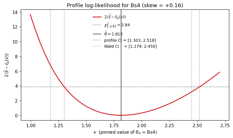
Three things to read off the plot:
The curve crosses the dashed \(\chi^2_{1,0.95}\) cutoff at the two red dotted lines — these are the profile-CI endpoints by construction (
_confint_profilesolves exactly \(2\,(\hat\ell - \ell_p(v)) - 3.84 = 0\) on each side viascipy.optimize.brentq).The right arm of the profile curve is visibly flatter than the left, which is exactly what the positive skew in the table records. A symmetric Wald paraboloid (blue dotted endpoints) misses this: the upper Wald endpoint sits inside the profile region while the lower Wald endpoint sits outside it.
On
Bs4, profile is shifted to the right relative to Wald — the baseline coefficient can take values further above \(\hat\theta\) than the symmetric approximation allows, because the only thing shrinking the right tail is the next-up boundary \(\theta_4\) has little neighbour to push against.
4. When to prefer each interval type#
Cost per parameter |
Honours asymmetry |
Robust to mis-specified link |
Robust to active constraints |
|
|---|---|---|---|---|
Wald |
one inversion of \(H\) at \(\hat\theta\) |
no |
no |
no — fails on monotonicity boundaries |
Sandwich |
one inversion of \(H\) + one \(s s^\top\) accumulation |
no |
yes |
no — same singular bread as Wald |
Profile |
\(\approx\) 10 constrained refits |
yes |
partially (still uses \(\ell\)) |
yes — refits under the pin |
Practical rules of thumb that follow from the table:
Default to Wald for fast triage and well-identified covariates (\(\beta_x\) above: all three methods agreed to 0.01).
Reach for sandwich when you suspect distributional mis-specification — heavy tails relative to the base distribution, residual heteroskedasticity not captured by
scaling=, etc. See also the`scaling-terms vignette<05_scaling_terms.ipynb>`__ for explicit modelling of heteroskedasticity, which often is the better answer than sandwiching.Reach for profile when (i) the Wald and sandwich CIs disagree on width despite the link looking right, (ii) the parameter sits near a boundary (Bernstein coefficients, scaling \(\gamma\) at the identification frontier, etc.), or (iii) you need to report a CI that you can defend as inversion of the LR test. Pay the extra ~10× cost on a
parm=[j]subset rather than the full vector unless \(p + q\) is small.
Profile and Wald CIs are R-parity tested against tram::Coxph / tram::BoxCox / tram::Colr in tests/test_confidence.py to rtol = 1e-3; the sandwich estimator is checked against sandwich::vcovHC(..., type = "HC0") in the same file.