Note

This page was generated from the notebook examples/05_scaling_terms.ipynb.

Scaling terms — heteroskedastic regression and non-proportional survival#

The default conditional transformation model adds covariates as an additive shift,

\[h(y \mid x_d) \;=\; h_0(y) + x_d^\top \beta,\]

which gives proportional hazards (Coxph), proportional odds (Colr), or a constant-variance Box-Cox. When the conditional distribution changes spread with the covariates — not just location — the shift model is mis-specified. mltpy’s scaling= kwarg mirrors R tram::*(scale = ~x_s) and multiplies the baseline by a strictly positive covariate-dependent factor:

\[h(y \mid x_d, x_s) \;=\; h_0(y)\, \exp\!\bigl(\tfrac{1}{2}\, x_s^\top \gamma\bigr) \;+\; x_d^\top \beta,\]

with \(\gamma\) unconstrained. See ADR 0002 for the parameter-vector layout, the monotonicity argument (scaling factor is positive, so \(h\) stays monotone in \(y\)), and the sign convention vs. R tram (γ is sign- and magnitude-aligned, including the conventional 0.5 factor on the exponent).

This vignette walks through two canonical uses of that machinery:

Heteroskedastic Box-Cox regression — variance of the response depends on a continuous covariate; the proportional model under-fits the heteroskedasticity and a likelihood-ratio test on \(\gamma\) rejects.
Non-proportional Cox survival — the shape of the survival curve changes with a covariate, so the curves spread (and cross) as \(t\) grows. Complements the interacting= route from 04_interacting_terms: different mechanism (multiplicative baseline scaling rather than tensor product), same kind of departure from proportionality.

[1]:

from pathlib import Path

import numpy as np
import matplotlib.pyplot as plt
from scipy.stats import chi2

import mltpy
from mltpy.variables import CensoredData

rng = np.random.default_rng(2026)
plt.rcParams["figure.dpi"] = 110
REF_DIR = Path("../../reference")  # repo-relative path to reference fixtures

1. Heteroskedastic Box-Cox regression#

We use the same n=100 dataset that the R-parity test in tests/test_tram_boxcox_scaling.py checks element-wise against tram::BoxCox(y ~ x_d | x_s). Loading it from reference/ rather than re-synthesising means the LR statistic we compute below is the same statistic R’s anova() would emit on this dataset — and the fixture below pins the expected value.

The data-generating process is

\[y_i \;=\; 1 + 0.5\, x^d_i + \varepsilon_i,\qquad \varepsilon_i \sim \mathcal{N}\!\bigl(0,\; e^{2\cdot 0.3\, x^s_i}\bigr),\]

so the residual variance grows with \(x_s\) — a textbook heteroskedasticity pattern.

[2]:

y = np.loadtxt(REF_DIR / "scaling_boxcox_normal_y.txt")
x_d = np.loadtxt(REF_DIR / "scaling_boxcox_normal_x_d.txt").reshape(-1, 1)
x_s = np.loadtxt(REF_DIR / "scaling_boxcox_normal_x_s.txt").reshape(-1, 1)
with open(REF_DIR / "scaling_boxcox_normal_support.txt") as fh:
    a, b = (float(t) for t in fh.read().split())

print(f"n={y.size}, support=({a:.2f}, {b:.2f})")
print(f"x_s range: [{x_s.min():+.2f}, {x_s.max():+.2f}]")
print(f"observed marginal sd of y: {y.std():.3f}")

n=100, support=(-1.77, 3.89)
x_s range: [-2.43, +2.87]
observed marginal sd of y: 0.994

Constant-variance baseline#

A standard BoxCox with x_d as a covariate. The transformation \(h\) depends only on \(y\), so the implied conditional distribution shares a single shape across all \(x_s\).

[3]:

null = mltpy.BoxCox(support=(a, b), order=5).fit(y, X=x_d)
print(null.summary())

Model:        BoxCox
Support:      (-1.76708573285841, 3.89175251100449)
Basis order:  5
Fitted:       Yes
Log-lik:      -129.3138
AIC:          272.6276
BIC:          290.8638
Converged:    Yes
n_restarts:   0

Coefficients:
          Estimate  Std. Error   z value   Pr(>|z|)
  X1       -0.5379      0.1175    -4.579  4.682e-06

Heteroskedastic Box-Cox via `scaling=`#

Passing scaling=x_s routes the model through the scaled-baseline likelihood path. The fitted parameter vector gains a \(\gamma\) block exposed as model.gamma_; the coefficient table in summary() adds a “Scaling coefficients” section so \(\gamma\) stands next to \(\beta\) for inference.

γ is reported in the same sign convention as R tram::BoxCox(..., scale=~x_s) — no flip required (ADR 0002, Decision 5).

[4]:

full = mltpy.BoxCox(support=(a, b), order=5, scaling=x_s).fit(y, X=x_d)
print(full.summary())
print(f"\ngamma_           = {full.gamma_}")
print(f"feature_names_scaling_ = {full.feature_names_scaling_}")

Model:        BoxCox
Support:      (-1.76708573285841, 3.89175251100449)
Basis order:  5
Fitted:       Yes
Log-lik:      -123.5189
AIC:          263.0378
BIC:          283.8791
Converged:    Yes
n_restarts:   0

Coefficients:
          Estimate  Std. Error   z value   Pr(>|z|)
  X1       -0.5608      0.1181    -4.749  2.043e-06
Scaling coefficients:
          Estimate  Std. Error   z value   Pr(>|z|)
  X1       -0.4573      0.1365    -3.351  0.0008054

gamma_           = [-0.45727429]
feature_names_scaling_ = ['X1']

Likelihood-ratio test against the constant-variance model#

Under \(H_0\!: \gamma = 0\) the deviance \(2(\ell_{\text{full}} - \ell_{\text{null}})\) is asymptotically \(\chi^2_{q_s}\). We compare against the reference value pinned by R’s anova(tram::BoxCox(...), tram::BoxCox(..., scale=~x_s)) on the same data — the parity fixture is regenerated by reference/generate_reference.R.

[5]:

ll_null = null.result_.log_likelihood
ll_full = full.result_.log_likelihood
df = full.n_free_params_ - null.n_free_params_
lr_stat = 2.0 * (ll_full - ll_null)
p_value = float(chi2.sf(lr_stat, df=df))

with open(REF_DIR / "scaling_vignette_boxcox_lr.txt") as fh:
    parts = fh.read().split()
lr_R = float(parts[0]); df_R = int(parts[1]); p_R = float(parts[2])

print(f"log-lik null : {ll_null:.4f}  (k={null.n_free_params_})")
print(f"log-lik full : {ll_full:.4f}  (k={full.n_free_params_})")
print(f"LR statistic : {lr_stat:.4f}  on {df} df,   p = {p_value:.4g}")
print(f"R reference  : {lr_R:.4f}  on {df_R} df,   p = {p_R:.4g}")
np.testing.assert_allclose(lr_stat, lr_R, rtol=1e-5, atol=1e-5)
print("\nparity OK — mltpy LR matches R anova at rtol=1e-5.")

log-lik null : -129.3138  (k=7)
log-lik full : -123.5189  (k=8)
LR statistic : 11.5899  on 1 df,   p = 0.0006631
R reference  : 11.5899  on 1 df,   p = 0.0006631

parity OK — mltpy LR matches R anova at rtol=1e-5.

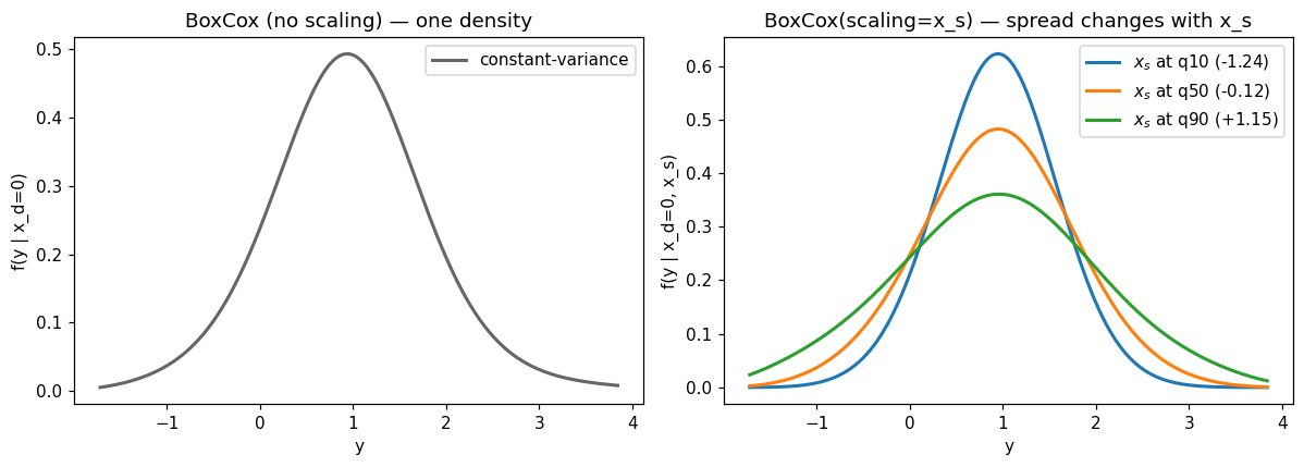
Conditional density at three \(x_s\) quantiles#

Holding \(x_d = 0\) fixed, we evaluate \(f(y \mid x_d=0, x_s)\) at the 10th, 50th, and 90th percentiles of the observed scaling covariate. The constant-variance baseline returns a single curve regardless of \(x_s\); the heteroskedastic fit visibly widens (and narrows) the conditional density as \(x_s\) changes.

[6]:

y_grid = np.linspace(a + 0.05, b - 0.05, 400)
xs_q = np.quantile(x_s.ravel(), [0.1, 0.5, 0.9])
colors = ["C0", "C1", "C2"]

fig, (ax_h, ax_f) = plt.subplots(1, 2, figsize=(11, 4))

# Left panel: the constant-variance model — one density for all x_s.
X_zero = np.zeros((y_grid.size, 1))
f_null = null.predict(y_grid, X_new=X_zero, what="density")
ax_h.plot(y_grid, f_null, lw=2, color="0.4", label="constant-variance")
ax_h.set_xlabel("y"); ax_h.set_ylabel("f(y | x_d=0)")
ax_h.set_title("BoxCox (no scaling) — one density")
ax_h.legend()

# Right panel: scaled fit — one density per x_s quantile.
for q, xs_val, c in zip([0.1, 0.5, 0.9], xs_q, colors):
    X_scale = np.full((y_grid.size, 1), xs_val)
    f_full = full.predict(y_grid, X_new=X_zero, X_scale_new=X_scale,
                          what="density")
    ax_f.plot(y_grid, f_full, lw=2, color=c,
              label=f"$x_s$ at q{int(q*100)} ({xs_val:+.2f})")
ax_f.set_xlabel("y"); ax_f.set_ylabel("f(y | x_d=0, x_s)")
ax_f.set_title("BoxCox(scaling=x_s) — spread changes with x_s")
ax_f.legend()
fig.tight_layout();

../_images/examples_05_scaling_terms_11_0.png

2. Non-proportional Cox survival#

Now we move to right-censored survival data. The scaled-baseline Cox model is

\[\log\bigl[-\log S(t \mid x_d, x_s)\bigr] \;=\; h_0(t)\, e^{0.5\, x_s\gamma} \;+\; x_d\,\beta,\]

i.e. the log-cumulative-hazard contribution of the baseline is scaled by \(e^{0.5 x_s\gamma}\). When \(\gamma \neq 0\) the proportional-hazards assumption fails: survival curves at different \(x_s\) values no longer differ by a constant vertical shift on the log-log scale, and can spread or cross.

We simulate from this model directly (so the fit can recover the non-PH structure) and visualise the resulting curves at three \(x_s\) quantiles.

[7]:

n_cox = 500
x_d_cox = rng.normal(size=n_cox)
x_s_cox = rng.normal(size=n_cox)
beta_true, gamma_true = -0.5, 1.2  # truth on the mltpy scale

# Direct inversion from the min-EV link:
#   S(t|x) = exp(-exp(h_0(t) * exp(0.5*x_s*γ) + x_d*β))
#   ⇒ Z = log(-log(1 - U)) ~ Gumbel_min
#   ⇒ h_0(T) = (Z - x_d*β) / exp(0.5*x_s*γ)
# Picking h_0(t) = log(t) gives an exponential-baseline Cox model
# whose shape is *modulated* by x_s.
U = rng.uniform(1e-5, 1 - 1e-5, size=n_cox)
Z = np.log(-np.log(1 - U))
h_target = (Z - x_d_cox * beta_true) / np.exp(0.5 * x_s_cox * gamma_true)
t = np.exp(h_target)

# Independent exponential censoring + a hard upper cap at b_max
# (treat clipped observations as right-censored).
cens = rng.exponential(scale=4.0, size=n_cox)
y_obs = np.minimum(t, cens)
event = (t <= cens).astype(int)
b_max = 8.0
y_obs = np.clip(y_obs, 1.1e-3, b_max - 1e-4)
event = np.where((t <= cens) & (t <= b_max), event, 0)
print(f"n={n_cox}, censoring={1 - event.mean():.1%}, "
      f"y in [{y_obs.min():.4f}, {y_obs.max():.3f}]")

a_cox, b_cox = 1e-3, b_max
cdata = CensoredData.right_censored(y_obs, (event == 0))

n=500, censoring=22.4%, y in [0.0011, 8.000]

Proportional-hazards baseline#

A standard Coxph with x_d as the only covariate — the textbook Cox proportional-hazards model with a smooth Bernstein baseline \(h_0(t)\). The shape of the implied survival curve does not depend on \(x_s\).

[8]:

ph = mltpy.Coxph(support=(a_cox, b_cox), order=6).fit(
    cdata, X=x_d_cox.reshape(-1, 1)
)
print(ph.summary())

Model:        Coxph
Support:      (0.001, 8.0)
Basis order:  6
Fitted:       Yes
Log-lik:      -515.9835
AIC:          1047.9671
BIC:          1081.6839
Converged:    Yes
n_restarts:   0

Coefficients:
          Estimate  Std. Error   z value   Pr(>|z|)
  X1       -0.4142      0.0520    -7.963  1.673e-15

Non-proportional fit via `scaling=`#

Coxph(..., scaling=x_s) adds the \(\gamma\) block; the baseline \(h_0(t)\) is multiplied by \(e^{0.5 x_s\gamma}\) per observation, which scales the log-cumulative hazard non-proportionally.

[9]:

np_cox = mltpy.Coxph(
    support=(a_cox, b_cox), order=6, scaling=x_s_cox.reshape(-1, 1)
).fit(cdata, X=x_d_cox.reshape(-1, 1))
print(np_cox.summary())
print(f"\ngamma_ (estimate vs truth γ={gamma_true}): {np_cox.gamma_}")

Model:        Coxph
Support:      (0.001, 8.0)
Basis order:  6
Fitted:       Yes
Log-lik:      -476.3271
AIC:          970.6542
BIC:          1008.5856
Converged:    Yes
n_restarts:   0

Coefficients:
          Estimate  Std. Error   z value   Pr(>|z|)
  X1       -0.4551      0.0526    -8.648  5.246e-18
Scaling coefficients:
          Estimate  Std. Error   z value   Pr(>|z|)
  X1        0.6872      0.0818     8.404  4.313e-17

gamma_ (estimate vs truth γ=1.2): [0.68716099]

Likelihood-ratio test against PH#

Same deviance recipe as Example 1: \(2(\ell_{\text{np}} - \ell_{\text{ph}})\) against a \(\chi^2_{q_s}\) reference.

[10]:

ll_ph = ph.result_.log_likelihood
ll_np = np_cox.result_.log_likelihood
df = np_cox.n_free_params_ - ph.n_free_params_
lr_stat = 2.0 * (ll_np - ll_ph)
p_value = float(chi2.sf(lr_stat, df=df))
print(f"log-lik PH      : {ll_ph:.3f}  (k={ph.n_free_params_})")
print(f"log-lik non-PH  : {ll_np:.3f}  (k={np_cox.n_free_params_})")
print(f"LR statistic    : {lr_stat:.2f} on {df} df,   p = {p_value:.3g}")

log-lik PH      : -515.984  (k=8)
log-lik non-PH  : -476.327  (k=9)
LR statistic    : 79.31 on 1 df,   p = 5.3e-19

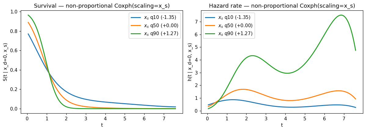
Spreading and crossing survival curves#

We evaluate \(S(t \mid x_d=0, x_s)\) over a fine \(t\)-grid at the 10th, 50th, and 90th percentiles of \(x_s\). Under PH the three curves would differ only by a constant vertical shift on the \(\log[-\log S]\) scale; under the scaled-baseline fit they spread as \(t\) grows and cross near the median follow-up — the canonical non-PH signature.

[11]:

t_grid = np.linspace(0.05, b_cox * 0.95, 200)
xs_q_cox = np.quantile(x_s_cox, [0.1, 0.5, 0.9])
colors = ["C0", "C1", "C2"]

fig, (ax_s, ax_h) = plt.subplots(1, 2, figsize=(11, 4))
X_zero = np.zeros((t_grid.size, 1))

for q, xs_val, c in zip([0.1, 0.5, 0.9], xs_q_cox, colors):
    X_scale = np.full((t_grid.size, 1), xs_val)
    S_np = np_cox.survival(t_grid, X=X_zero, X_scale=X_scale)
    h_np = np_cox.hazard(t_grid, X=X_zero, X_scale=X_scale)
    ax_s.plot(t_grid, S_np, lw=2, color=c,
              label=f"$x_s$ q{int(q*100)} ({xs_val:+.2f})")
    ax_h.plot(t_grid, h_np, lw=2, color=c,
              label=f"$x_s$ q{int(q*100)} ({xs_val:+.2f})")

ax_s.set_xlabel("t"); ax_s.set_ylabel("S(t | x_d=0, x_s)")
ax_s.set_title("Survival — non-proportional Coxph(scaling=x_s)")
ax_s.legend()
ax_h.set_xlabel("t"); ax_h.set_ylabel("h(t | x_d=0, x_s)")
ax_h.set_title("Hazard rate — non-proportional Coxph(scaling=x_s)")
ax_h.legend()
fig.tight_layout();

../_images/examples_05_scaling_terms_21_0.png

Takeaways#

The scaling= kwarg on BoxCox / Coxph / Colr / Lm / Survreg mirrors R tram::*(scale = ~x_s) and multiplies the baseline by \(e^{0.5 x_s \gamma}\). γ is unconstrained — monotonicity in \(y\) is inherited from \(h_0\) because the scaling factor is strictly positive (ADR 0002, Decision 3).
The fitted model exposes gamma_ and feature_names_scaling_; summary() adds a Scaling coefficients block with Wald standard errors and p-values for \(\gamma\).
Sign convention is identical to R for \(\gamma\) — no flip when porting tram fits. (β is still negated; the summary() tabulation handles that for you.)
predict(...) and the convenience methods survival(...) / hazard(...) take an extra X_scale_new= / X_scale= argument on scaled fits.
Likelihood-ratio tests on \(\gamma\) work the same way they do for any nested-model comparison: deviance \(2\Delta\ell\) on \(q_s\) df.
Combining scaling= with interacting= (tensor-product baseline) is out of scope for v0.4 and raises ValueError; if you need and shape-on-y and and spread-on-x, fit them as two separate models and compare via deviance. See 04_interacting_terms for the tensor-product route on its own.

Scaling terms — heteroskedastic regression and non-proportional survival#

1. Heteroskedastic Box-Cox regression#

Constant-variance baseline#

Heteroskedastic Box-Cox via scaling=#

Likelihood-ratio test against the constant-variance model#

Conditional density at three \(x_s\) quantiles#

2. Non-proportional Cox survival#

Proportional-hazards baseline#

Non-proportional fit via scaling=#

Likelihood-ratio test against PH#

Spreading and crossing survival curves#

Takeaways#

Heteroskedastic Box-Cox via `scaling=`#

Non-proportional fit via `scaling=`#