Note
This page was generated from the notebook examples/02_survival_analysis.ipynb.
Survival analysis with Coxph#
mltpy.Coxph fits a proportional-hazards model in which the baseline log-cumulative-hazard is modelled as a flexible, monotone Bernstein polynomial and the link function is the minimum-extreme-value distribution. With covariates entering linearly, this is equivalent to the classical Cox proportional-hazards model, but the baseline distribution is estimated smoothly rather than left fully non-parametric.
This vignette reproduces the Cox-PH illustration from Hothorn (2020) on synthetic right-censored data and compares the estimated survival curve to the Kaplan-Meier estimate from lifelines.
lifelines is an optional dependency: install with
pip install "mltpy[examples]".
[1]:
import numpy as np
import matplotlib.pyplot as plt
from lifelines import KaplanMeierFitter

import mltpy

rng = np.random.default_rng(0)
plt.rcParams["figure.dpi"] = 110
Data-generating process#
250 event times from \(T\sim\text{Exp}(\text{scale}=2)\), observed under independent uniform right-censoring. The censoring window is tuned to a ~30 % censoring rate, a realistic setting for observational follow-up studies.
mltpy expects a CensoredData container with the convention censored=True when the event is not observed.
[2]:
n = 250
t_event = rng.exponential(scale=2.0, size=n)
c = rng.uniform(0.8, 5.0, size=n)
y_obs = np.minimum(t_event, c)
event = t_event <= c         # True -> exact observation
censored = ~event            # mltpy: True -> right-censored
print(f"censoring rate = {censored.mean():.0%}")
print(f"observed time range: [{y_obs.min():.3f}, {y_obs.max():.3f}]")
censoring rate = 33%
observed time range: [0.003, 4.891]
[3]:
cd = mltpy.CensoredData.right_censored(y_obs, censored)

support = (float(y_obs.min()) * 0.5, float(y_obs.max()) + 0.5)
model = mltpy.Coxph(support=support, order=6)
model.fit(cd)
print(model.summary())
Model:        Coxph
Support:      (0.001287750334822838, 5.390734500379891)
Basis order:  6
Fitted:       Yes
Log-lik:      -330.5756
AIC:          675.1511
BIC:          699.8014
Converged:    Yes
n_restarts:   0
Kaplan-Meier reference#
The non-parametric Kaplan-Meier estimator is the standard baseline for right-censored survival data. It serves as the reference against which the smooth Coxph estimate is compared. lifelines expects the event indicator — the complement of censored.
[4]:
kmf = KaplanMeierFitter()
kmf.fit(durations=y_obs, event_observed=event.astype(int), label="Kaplan-Meier")
km_median = kmf.median_survival_time_
ctm_median = model.predict(np.array([0.5]), what="quantile")[0]
true_median = 2.0 * np.log(2)
print(f"true median     : {true_median:.3f}")
print(f"Kaplan-Meier    : {km_median:.3f}")
print(f"mltpy Coxph     : {ctm_median:.3f}")
true median     : 1.386
Kaplan-Meier    : 1.596
mltpy Coxph     : 1.555
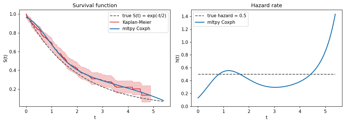
Survival and hazard curves#
[5]:
t_grid = np.linspace(support[0] + 1e-3, support[1] - 1e-3, 400)
S_ctm = model.survival(t_grid)
h_ctm = model.hazard(t_grid)
# Truth: Exp(scale=2) has S(t) = exp(-t/2), hazard 0.5.
S_true = np.exp(-t_grid / 2.0)
h_true = np.full_like(t_grid, 0.5)

fig, (ax_s, ax_h) = plt.subplots(1, 2, figsize=(11, 4))

ax_s.plot(t_grid, S_true, "--", color="0.3", label="true S(t) = exp(-t/2)")
kmf.plot_survival_function(ax=ax_s, color="C3", ci_show=True)
ax_s.plot(t_grid, S_ctm, label="mltpy Coxph", lw=2, color="C0")
ax_s.set_xlabel("t")
ax_s.set_ylabel("S(t)")
ax_s.set_title("Survival function")
ax_s.legend()

ax_h.plot(t_grid, h_true, "--", color="0.3", label="true hazard = 0.5")
ax_h.plot(t_grid, h_ctm, label="mltpy Coxph", lw=2, color="C0")
ax_h.set_xlabel("t")
ax_h.set_ylabel("h(t)")
ax_h.set_title("Hazard rate")
ax_h.set_ylim(0, 1.5)
ax_h.legend()
fig.tight_layout();
Takeaways#
The Coxph estimate tracks the Kaplan-Meier survival curve closely, but is smooth — it does not have the staircase pattern of KM and returns finite values everywhere inside the support.
Because the fit is smooth, the hazard rate is directly available via
model.hazard(t). KM provides no hazard estimate without further kernel smoothing.The median survival time recovered by mltpy sits between the truth \(2\ln 2 \approx 1.386\) and the KM estimate — both are consistent at \(n=250\) with ~30 % censoring.
Coxphaccepts covariates throughfit(cd, X=X)exactly likeMLT; the hazard ratios appear in the trailing entries ofmodel.theta_.