Note
This page was generated from the notebook examples/03_regression_covariates.ipynb.
Conditional transformation model with covariates#
When a conditioning covariate matrix \(X\) is supplied, mltpy fits the conditional distribution
where the Bernstein component \(B_k(y)\,\theta\) absorbs the shape of the response distribution and \(x^{\top}\beta\) shifts it on the latent normal scale.
Unlike ordinary linear regression, nothing here is restricted to the mean: the model describes the entire conditional distribution, so we can extract the CDF, density, or any quantile at any covariate value. This is the conditional transformation model of Hothorn, Kneib & Bühlmann (2014).
In this vignette we:
Simulate a heteroscedastic two-covariate regression problem.
Fit
mltpy.MLTwithXpassed tofit.Compare conditional densities at three representative covariate values against the Gaussian densities implied by OLS.
[1]:
import numpy as np
import matplotlib.pyplot as plt
from scipy import stats

import mltpy

rng = np.random.default_rng(0)
plt.rcParams["figure.dpi"] = 110
Heteroscedastic DGP#
\(X_1, X_2 \sim \mathcal{N}(0, 1)\) independently, and
The residual variance grows with \(|X_1|\), so the conditional distribution is not a location shift of a single shape — exactly the regime in which the naive Gaussian regression fails.
[2]:
n = 300
X = rng.standard_normal((n, 2))
eta = 1.0 + 0.8 * X[:, 0] - 0.5 * X[:, 1]
sd = 0.3 + 0.2 * np.abs(X[:, 0])
y = eta + sd * rng.standard_normal(n)
print(f"y range: [{y.min():.2f}, {y.max():.2f}]")
y range: [-2.33, 4.10]
Fit the conditional transformation model#
[3]:
support = (float(y.min()) - 1.0, float(y.max()) + 1.0)
model = mltpy.MLT(order=5, support=support)
model.fit(y, X=X)

p = 5 + 1
beta = model.theta_[p:]
print(f"converged: {model.result_.converged}")
print(f"log-likelihood: {model.result_.log_likelihood:.2f}")
print(f"beta = {beta}   (true shifts: [-0.8/sd, +0.5/sd] on latent scale)")
converged: True
log-likelihood: -167.26
beta = [-1.91573912  1.15235702]   (true shifts: [-0.8/sd, +0.5/sd] on latent scale)
Conditional CDF and density at three representative \(x\) values#
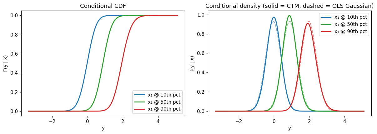
We pick \(x_1\) at the 10th, 50th, and 90th empirical percentile with \(x_2\) held at 0 to isolate the heteroscedastic axis. For each value we compute the CTM conditional distribution and the Gaussian distribution implied by OLS with constant residual variance.
[4]:
X_design = np.column_stack([np.ones(n), X])
coefs_ols, *_ = np.linalg.lstsq(X_design, y, rcond=None)
resid = y - X_design @ coefs_ols
sigma_ols = resid.std(ddof=X_design.shape[1])
print(f"OLS coefficients (intercept, x1, x2): {coefs_ols}")
print(f"OLS residual SD (assumed constant):   {sigma_ols:.3f}")
OLS coefficients (intercept, x1, x2): [ 0.99732622  0.8071613  -0.48716702]
OLS residual SD (assumed constant):   0.428
[5]:
x1_values = np.quantile(X[:, 0], [0.10, 0.50, 0.90])
colors = ["C0", "C2", "C3"]
labels = ["x₁ @ 10th pct", "x₁ @ 50th pct", "x₁ @ 90th pct"]

y_grid = np.linspace(support[0] + 1e-3, support[1] - 1e-3, 400)

fig, (ax_cdf, ax_pdf) = plt.subplots(1, 2, figsize=(11, 4))

for x1, col, lbl in zip(x1_values, colors, labels):
    x_fixed = np.array([x1, 0.0])
    X_rep = np.tile(x_fixed, (len(y_grid), 1))
    cdf = model.predict(y_grid, X_new=X_rep, what="distribution")
    pdf = model.predict(y_grid, X_new=X_rep, what="density")
    ax_cdf.plot(y_grid, cdf, color=col, lw=2, label=lbl)
    ax_pdf.plot(y_grid, pdf, color=col, lw=2, label=lbl)

    # OLS-implied Gaussian conditional density at the same x
    mu_ols = coefs_ols[0] + coefs_ols[1] * x1 + coefs_ols[2] * 0.0
    ax_pdf.plot(
        y_grid,
        stats.norm.pdf(y_grid, mu_ols, sigma_ols),
        "--",
        color=col,
        alpha=0.6,
    )

ax_cdf.set_xlabel("y")
ax_cdf.set_ylabel("F(y | x)")
ax_cdf.set_title("Conditional CDF")
ax_cdf.legend(loc="lower right")

ax_pdf.set_xlabel("y")
ax_pdf.set_ylabel("f(y | x)")
ax_pdf.set_title("Conditional density (solid = CTM, dashed = OLS Gaussian)")
ax_pdf.legend(loc="upper right")

fig.tight_layout();
Takeaways#
At moderate \(x_1\) the CTM and OLS densities roughly coincide: when the DGP’s conditional noise is close to its mean level, a homoscedastic Gaussian is not grossly wrong.
At extreme \(x_1\) the CTM density is visibly narrower or wider than the fixed-SD OLS Gaussian — the model recovers the heteroscedasticity directly from the likelihood, without any explicit variance model.
The same fitted object answers conditional-quantile queries: use
model.predict(np.array([0.1, 0.5, 0.9]), X_new=..., what="quantile")to obtain conditional prediction bands.For censored responses the same covariate path is available through
mltpy.Coxph(...).fit(CensoredData, X=X).