Note

This page was generated from the notebook examples/04_interacting_terms.ipynb.

Interacting terms — non-proportional hazards and stratified baselines#

Conditional transformation models (CTMs) usually split the dependence of the response on the covariates into a baseline transformation \(h_0(y)\) and an additive shift \(x^\top\beta\):

\[h(y \mid x) \;=\; h_0(y) + x^\top \beta,\]

the assumption that yields proportional hazards (Coxph), proportional odds (Colr), or a covariate-shifted Gaussian (BoxCox). When that assumption fails — when the shape of the conditional distribution changes with \(x\), not just its location — the shift model is mis-specified. mltpy’s :class:~mltpy.basis.InteractionBasis replaces the additive structure with a tensor product,

\[h(y \mid x) \;=\; \bigl(a(y) \otimes b(x)\bigr)^{\!\top} \mathrm{vec}(\Theta),\]

so the transformation itself depends on \(x\). See ADR 0001 for the parameter-vector layout and monotonicity strategy.

This vignette walks through two canonical uses of that machinery:

Stratified Box-Cox — different baseline transformations per stratum (Bernstein-y \(\otimes\) one-hot-x).
Non-proportional Cox — survival curves that cross under a continuous covariate (Bernstein-y \(\otimes\) Bernstein-x).

For each example we fit the model, compare it against the proportional baseline via a likelihood-ratio test, and plot the conditional CDF, density, survival and hazard.

[1]:

import numpy as np
import matplotlib.pyplot as plt
from scipy.stats import chi2

import mltpy
from mltpy.basis import BernsteinBasis, OneHotBasis

rng = np.random.default_rng(0)
plt.rcParams["figure.dpi"] = 110

1. Stratified Box-Cox#

We simulate three groups whose conditional distributions disagree both in location and in shape, so the proportional Box-Cox model (\(h(y) + x^\top\beta \sim \mathcal{N}(0,1)\)) cannot fit them.

Stratum 0 — \(\mathcal{N}(\mu=2,\,\sigma=0.6)\) (sharply peaked).
Stratum 1 — \(\mathcal{N}(\mu=4,\,\sigma=1.2)\) (medium spread).
Stratum 2 — \(\log\mathcal{N}(\mu=1.4,\,\sigma=0.45)\) (right-skewed).

The third stratum is deliberately non-Gaussian — a global Box-Cox would force a single \(h\) to fit all three shapes simultaneously, and the skewed stratum is the one that pays for the compromise.

[2]:

n_per = 250
K = 3
stratum = np.repeat(np.arange(K), n_per).astype(float)
y_s0 = rng.normal(loc=2.0, scale=0.6, size=n_per)
y_s1 = rng.normal(loc=4.0, scale=1.2, size=n_per)
y_s2 = rng.lognormal(mean=1.4, sigma=0.45, size=n_per)
y = np.concatenate([y_s0, y_s1, y_s2])

a = float(y.min()) - 0.25
b = float(y.max()) + 0.25
print(f"n={y.size},  support=({a:.2f}, {b:.2f}),  K={K}")

n=750,  support=(-0.93, 12.15),  K=3

Proportional baseline (shift model)#

A standard BoxCox with the stratum index entered as a covariate. This is the proportional reference model: a single baseline transformation \(h_0\) is shifted by \(x^\top\beta\) — it cannot change shape between strata.

[3]:

X_shift = np.zeros((y.size, K - 1), dtype=float)
for k in range(1, K):
    X_shift[stratum == k, k - 1] = 1.0

shift = mltpy.BoxCox(support=(a, b), order=6).fit(y, X=X_shift)
print(shift.summary())

Model:        BoxCox
Support:      (-0.929306076065207, 12.146664193459673)
Basis order:  6
Fitted:       Yes
Log-lik:      -1185.7967
AIC:          2389.5935
BIC:          2431.1741
Converged:    Yes
n_restarts:   0

Coefficients:
          Estimate  Std. Error   z value   Pr(>|z|)
  X1       -1.8205      0.1048   -17.364  1.549e-67
  X2       -1.9785      0.1043   -18.978  2.581e-80

Fully-interacting model (stratified baseline)#

Bernstein-y \(\otimes\) one-hot-x: each stratum gets its own baseline Bernstein coefficients, but they share a degree and a support. The column-wise monotonicity constraint guarantees that \(h\) is non-decreasing in \(y\) separately within every stratum.

[4]:

y_basis = BernsteinBasis(order=6, support=(a, b))
x_basis = OneHotBasis(K=K)
ib = mltpy.InteractionBasis(y_basis=y_basis, x_basis=x_basis)

interact = mltpy.ConditionalTransformationModel(
    basis=ib,
    base_distribution="normal",
    censoring=mltpy.CensoringType.NONE,
    optimizer_config=mltpy.OptimizerConfig(random_state=0),
).fit(y, X=stratum.astype(int))
print(interact)

ConditionalTransformationModel(order=6, censoring=NONE, fitted=True, ll=-1118.94)

Likelihood-ratio test against the shift model#

Under \(H_0\) (proportional shift) the LR statistic \(2(\ell_{\text{interact}} - \ell_{\text{shift}})\) is asymptotically \(\chi^2\) with df equal to the difference in free parameters.

[5]:

ll_shift = shift.result_.log_likelihood
ll_full = interact.result_.log_likelihood
df = interact.n_free_params_ - shift.n_free_params_
lr = 2.0 * (ll_full - ll_shift)
p_value = float(chi2.sf(lr, df=df))
print(f"log-lik shift    : {ll_shift:.3f}  (k={shift.n_free_params_})")
print(f"log-lik interact : {ll_full:.3f}  (k={interact.n_free_params_})")
print(f"LR statistic     : {lr:.2f} on {df} df,  p = {p_value:.2e}")

log-lik shift    : -1185.797  (k=9)
log-lik interact : -1118.938  (k=21)
LR statistic     : 133.72 on 12 df,  p = 1.11e-22

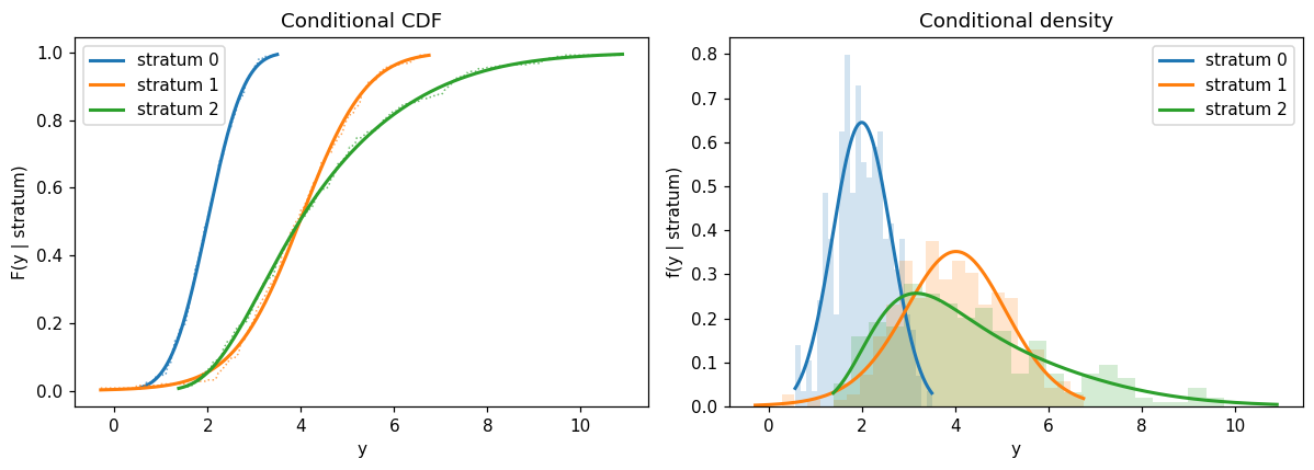
Conditional CDF and density per stratum#

The interacting model returns one conditional curve per requested covariate row. We evaluate \(F(y \mid k)\) and \(f(y \mid k)\) over a fine \(y\)-grid for \(k = 0, 1, 2\) and overlay the empirical CDF / a kernel density estimate from each stratum for context.

[6]:

fig, (ax_cdf, ax_pdf) = plt.subplots(1, 2, figsize=(11, 4))

colors = ["C0", "C1", "C2"]
for k in range(K):
    yk = y[stratum == k]
    lo, hi = float(np.quantile(yk, 0.005)), float(np.quantile(yk, 0.995))
    y_grid = np.linspace(lo, hi, 300)
    xk = np.full(y_grid.shape, k, dtype=int)
    cdf_k = interact.predict(y_grid, X_new=xk, what="distribution")
    pdf_k = interact.predict(y_grid, X_new=xk, what="density")

    ecdf = np.searchsorted(np.sort(yk), y_grid, side="right") / yk.size

    ax_cdf.plot(y_grid, cdf_k, color=colors[k], lw=2, label=f"stratum {k}")
    ax_cdf.plot(y_grid, ecdf, color=colors[k], lw=1, ls=":", alpha=0.7)
    ax_pdf.plot(y_grid, pdf_k, color=colors[k], lw=2, label=f"stratum {k}")
    ax_pdf.hist(yk, bins=25, density=True, color=colors[k], alpha=0.2, range=(lo, hi))

ax_cdf.set_xlabel("y"); ax_cdf.set_ylabel("F(y | stratum)")
ax_cdf.set_title("Conditional CDF"); ax_cdf.legend()
ax_pdf.set_xlabel("y"); ax_pdf.set_ylabel("f(y | stratum)")
ax_pdf.set_title("Conditional density"); ax_pdf.legend()
fig.tight_layout();

../_images/examples_04_interacting_terms_11_0.png

Quantile prediction#

predict(..., what="quantile") inverts \(h(\,\cdot\,\mid x)\) row-by-row on the interaction path — the same grid+spline machinery used for the non-proportional Cox example below. The conditional medians track the Gaussian/lognormal medians of each stratum.

[7]:

probs = np.array([0.5, 0.5, 0.5])
x_pred = np.array([0, 1, 2], dtype=int)
med_hat = interact.predict(probs, X_new=x_pred, what="quantile")
med_true = np.array([2.0, 4.0, np.exp(1.4)])  # lognormal median = exp(mu)
for k in range(K):
    print(
        f"stratum {k}:  mltpy median = {med_hat[k]:.3f}"
        f"   true median = {med_true[k]:.3f}"
    )

stratum 0:  mltpy median = 1.997   true median = 2.000
stratum 1:  mltpy median = 3.976   true median = 4.000
stratum 2:  mltpy median = 3.969   true median = 4.055

2. Non-proportional Cox — crossing survival curves#

Now we leave the categorical setting and use a continuous covariate. We simulate survival times whose hazard shape depends on \(x\): low-\(x\) observations have a decreasing hazard (Weibull shape \(< 1\), frailty-like early failure) while high-\(x\) observations have an increasing hazard (Weibull shape \(> 1\), ageing). The medians are similar by construction, so the survival curves cross in the middle of the support — exactly the textbook violation of the proportional-hazards assumption.

We then fit a non-proportional Coxph using interacting=BernsteinBasis(...), which expands the baseline log-cumulative-hazard \(h\) over both \(t\) and \(x\) simultaneously.

[8]:

n_cox = 600
x_cont = rng.uniform(0.0, 1.0, size=n_cox)
shape = 0.8 + 1.4 * x_cont  # 0.8 at x=0  ->  2.2 at x=1
scale = 2.0  # common scale; all S(t | x) curves cross at t = scale
u = rng.uniform(size=n_cox)
t = scale * (-np.log(u)) ** (1.0 / shape)
support_t = (float(t.min()) * 0.5, float(t.max()) + 0.5)
print(f"n={n_cox},  t in [{t.min():.3f}, {t.max():.3f}],  shape in [{shape.min():.2f}, {shape.max():.2f}]")

n=600,  t in [0.004, 13.890],  shape in [0.80, 2.19]

Proportional baseline#

A standard Coxph with \(x\) as a single-column covariate — the classical Cox model with a smooth Bernstein baseline.

[9]:

prop = mltpy.Coxph(support=support_t, order=6).fit(t, X=x_cont.reshape(-1, 1))
print(prop.summary())

Model:        Coxph
Support:      (0.0021859245671776496, 14.389615100396629)
Basis order:  6
Fitted:       Yes
Log-lik:      -1018.6470
AIC:          2053.2939
BIC:          2088.4694
Converged:    Yes
n_restarts:   0

Coefficients:
          Estimate  Std. Error   z value   Pr(>|z|)
  X1        0.4039      0.1459     2.768   0.005632

Non-proportional fit#

Passing interacting=BernsteinBasis(order=q-1, support=(0,1)) routes the model through the tensor-product likelihood path; the time-basis stays at order 6 on the original support. Only exact (non-censored) times are supported on the interaction path in the current release; the censoring argument set internally to RIGHT is ignored when no CensoredData container is supplied.

[10]:

x_basis_cox = BernsteinBasis(order=3, support=(0.0, 1.0))
npcox = mltpy.Coxph(
    support=support_t,
    order=6,
    optimizer_config=mltpy.OptimizerConfig(random_state=0),
    interacting=x_basis_cox,
).fit(t, X=x_cont)
ll_prop = prop.result_.log_likelihood
ll_np = npcox.result_.log_likelihood
df = npcox.n_free_params_ - prop.n_free_params_
lr = 2.0 * (ll_np - ll_prop)
p_value = float(chi2.sf(lr, df=df))
print(f"log-lik proportional     : {ll_prop:.3f}  (k={prop.n_free_params_})")
print(f"log-lik non-proportional : {ll_np:.3f}  (k={npcox.n_free_params_})")
print(f"LR statistic             : {lr:.2f} on {df} df,  p = {p_value:.2e}")

log-lik proportional     : -1018.647  (k=8)
log-lik non-proportional : -992.194  (k=28)
LR statistic             : 52.91 on 20 df,  p = 8.39e-05

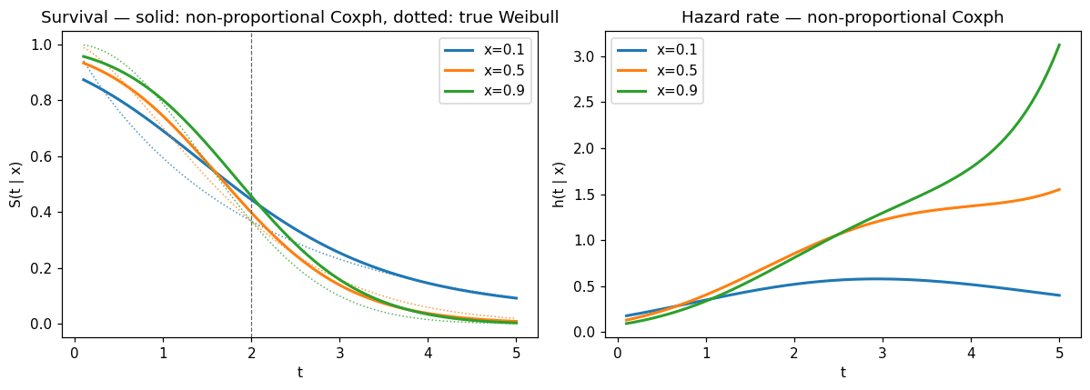
Crossing survival curves#

We evaluate \(S(t \mid x)\) for three representative covariate values (\(x = 0.1, 0.5, 0.9\)), overlay the true Weibull survival, and confirm visually that the curves cross.

[11]:

t_grid = np.linspace(0.1, 5.0, 300)
x_reps = np.array([0.1, 0.5, 0.9])
fig, (ax_s, ax_h) = plt.subplots(1, 2, figsize=(11, 4))

for i, xv in enumerate(x_reps):
    xv_grid = np.full_like(t_grid, xv)
    S_np = npcox.survival(t_grid, X=xv_grid)
    h_np = npcox.hazard(t_grid, X=xv_grid)
    shape_v = 0.8 + 1.4 * xv
    S_true = np.exp(-((t_grid / scale) ** shape_v))
    color = f"C{i}"
    ax_s.plot(t_grid, S_np, color=color, lw=2, label=f"x={xv}")
    ax_s.plot(t_grid, S_true, color=color, lw=1, ls=":", alpha=0.8)
    ax_h.plot(t_grid, h_np, color=color, lw=2, label=f"x={xv}")

ax_s.axvline(scale, color="0.4", lw=0.8, ls="--")
ax_s.set_xlabel("t"); ax_s.set_ylabel("S(t | x)")
ax_s.set_title("Survival — solid: non-proportional Coxph, dotted: true Weibull")
ax_s.legend()
ax_h.set_xlabel("t"); ax_h.set_ylabel("h(t | x)")
ax_h.set_title("Hazard rate — non-proportional Coxph")
ax_h.legend()
fig.tight_layout();

../_images/examples_04_interacting_terms_21_0.png

Quantile prediction on the interaction model#

predict(..., what="quantile") on the non-proportional Coxph uses the row-wise bracket from #67: for each requested probability/\(x\) pair the bracket is derived from the per-row \(h(a, x)\) and \(h(b, x)\) rather than the global Bernstein endpoints. Below we recover the median survival time at three covariate values.

[12]:

probs = np.full_like(x_reps, 0.5)
med = npcox.predict(probs, X_new=x_reps, what="quantile")
med_true = scale * (np.log(2.0)) ** (1.0 / (0.8 + 1.4 * x_reps))
for xv, m_hat, m_t in zip(x_reps, med, med_true):
    print(f"x={xv}:  mltpy median = {m_hat:.3f}   true Weibull median = {m_t:.3f}")

x=0.1:  mltpy median = 1.767   true Weibull median = 1.354
x=0.5:  mltpy median = 1.711   true Weibull median = 1.566
x=0.9:  mltpy median = 1.884   true Weibull median = 1.674

Takeaways#

An :class:~mltpy.basis.InteractionBasis replaces the additive shift \(h_0(y) + x^\top\beta\) with the tensor product \((a(y) \otimes b(x))^\top \mathrm{vec}(\Theta)\), letting the shape of the conditional distribution change with \(x\).
For stratified (categorical) covariates the natural x-basis is :class:~mltpy.basis.OneHotBasis; for continuous covariates use :class:~mltpy.basis.BernsteinBasis (or :class:~mltpy.basis.OrdinalBasis for ordered categories). All three are non-negative partitions of unity, the condition needed for the closed-form column-wise monotonicity constraint.
The fitted interaction model exposes the standard prediction surface (distribution, density, survivor, hazard, quantile) and works with simulate and plot as documented in ADR 0001.
The likelihood-ratio test against the proportional baseline is the practical way to decide whether the extra flexibility is justified for a given dataset.